
Как сделать саммари в excel
This is the third article of the five-part series on Data Analysis in Excel. In this section, I will show you how to use the Scenario Manager in Excel.
Other articles in this series:
Watch Video – Scenario Manager in Excel
Scenario Manager in Excel can be the tool of choice when you have multiple variables, and you want to see the effect on the final result when these variables change.
Suppose you have a dataset as shown below and you want to calculate the profit value:

The Profit value is dependent on 3 variables – Sale Quantity, Price per Unit, and the Variable Cost per Unit. Here is the formula I have used to calculate the profit:
The idea is to see how this final result changes when we change these dependent variables.
As shown in the first 2 articles of this series, if you only have one or two variables changing, you can create one variable or two-variable data table. But if you have 3 or variables that can change then scenario manager is the way to go.
Setting up Scenario Manager in Excel

This creates the Worst Case scenario for this data set. You can similarly follow these steps and create multiple scenarios (for example, Worst Case, Realistic, Best Case).
Once you have created all the scenarios, you can view the result from each of the scenarios by simply double-clicking on any of the scenarios. As you double click, the values would change based on that scenario.
Additionally, you can also create a summary of all the scenarios.
Create a Summary of all the Scenarios
Scenario manager in Excel is a great tool when you need to do sensitivity analysis. Simply create scenarios and a summary can be generated instantly, giving you a complete comparative overview.
Download File… Try it yourself You May Also Like the Following Excel Tutorials:
In this video, I want to show you how to build a quick summary table using the COUNTIF and SUMIF functions.
Here we have a sample set of data that shows t-shirt sales.
You can see we have columns for date, item, color, and amount.
So let's break this data down by color.
Now, before we start, I want to mention that Pivot Tables would be an excellent way to summarize this data, but you can certainly use formulas for basic summaries, and that's what I'm going to demonstrate here.
First, I'm going to name the Color and Amount columns in the data. Now, this isn't necessary, but naming these ranges means I won't need to use absolute addresses later, and it will make the formulas really short and easy to read.
Now, in our summary table, we need a list of unique colors. To build this list, I'll copy the full list, then use the Remove Duplicates command in Excel.
If you just have a few items in a list, there's no need to use Remove Duplicates. But it's a great way to build a clean list of unique values when you're working with unfamiliar data.
Now I'll add the first formula. COUNTIF needs a range and a criteria. Since we're counting colors, the range is the color column.
Next, we need a criteria, and that's where our list of colors comes in. We already have the colors in a list in our table, so I can just point to that column and pick up the reference. When I hit Enter, and copy the formula down, we have a count for each color.
Now let's extend this summary table to include amounts.
In this case, we'll need to use the SUMIF function. As before, I need to provide Color as the range, then pick up the name of the color as a cell reference in our table.
Then we need to provide the range to sum, which is the Amounts column.
When I copy the formula down the table, we have a breakdown of amount by color.
Now, to finish things off, I can copy formatting from the source table to the summary table using Paste Special.
So there you have it; we have our summary table. And, if I change some of the source data, you'll see the summary table update instantly.
Сводный отчет Excel резюмирует или суммирует значения, хранящиеся на множестве других листов в книге. Лучший способ научиться создавать сводный рабочий лист - это пройти через процедуру его создания (под названием «Общий прогнозируемый доход») для вымышленной компании.
В связи с этим, как сделать сводку в Excel?
Измените функцию сводки
- Щелкните правой кнопкой мыши ячейку в поле «Значение», которое вы хотите изменить.
- Во всплывающем меню нажмите «Суммировать значения по».
- Щелкните функцию сводки, которую вы хотите использовать.
Что касается этого, является ли Excel инструментом отчетности?
Что такое Excel Reporting Tool? Инструменты отчетности Excel расширенные программы для работы с электронными таблицами, предназначенный для удобного создания отчетов. Интерфейс похож на Excel. Итак, способ присвоения имени ячейке, установки атрибутов ячейки, редактирования ячейки такой же, как и в Excel.
Кроме того, как написать хорошее резюме для отчета?
5 советов по написанию сводного отчета
- Сделайте набросок отчета до начала встречи или телефонного звонка. …
- Включите только ключевые моменты мероприятия. …
- Будьте лаконичны. …
- Для большей ясности используйте маркеры. …
- Перечитайте свой отчет!
Как мне написать резюме?
4 совета по написанию хорошего резюме
- Найдите главную идею. Полезное резюме сводит исходный материал к самому важному, чтобы проинформировать читателя. …
- Будьте краткими. Резюме - это не переписывание, это краткое изложение исходного текста. …
- Пишите без осуждения. …
- Убедитесь, что он течет.
Как сделать сводную таблицу?
Вот шаги, через которые они проходят.
- Начало работы - скопируйте данные.
- Ваша первая сводная таблица.
- Добавьте в таблицу строки и значения.
- Обобщить по: COUNT.
- Добавить еще одно поле к значениям.
В чем плох Excel?
Excel - это ужасное место для хранения и извлечения данных. Он предназначен для анализа данных. У вас будет электронная таблица с множеством вложенных листов (вкладок). Часто одни и те же данные вводятся в разные места во многих разных таблицах.
Какие формулы в Excel?
Семь основных формул Excel для вашего рабочего процесса
- = СУММ (число1; [число2];…)…
- = СУММ (A2: A8) - простой выбор, который суммирует значения столбца.
- = СУММ (A2: A8) / 20 - показывает, что вы также можете превратить свою функцию в формулу. …
- = СРЕДНИЙ (число1; [число2];…)…
- = СРЕДНЕЕ (B2: B11) - показывает простое среднее значение, также похожее на (СУММ (B2: B11) / 10)
Чем хорош Excel?
Excel имеет очень простые в использовании функции построения диаграмм по сравнению с другим программным обеспечением, а также несколько полезных встроенных функций. … Excel хорош еще и потому, что вы есть возможность вырезать и вставлять в отчеты. Большинство людей пишут отчеты в Word, поэтому можно легко вырезать и вставлять данные или диаграммы из Excel в Word.
Что такое сводный пример?
Определение резюме - это заявление, в котором излагаются основные моменты. Пример резюме своего рода обзор того, что произошло на встрече. … Резюме определяется как быстрый или краткий обзор того, что произошло. Примером резюме является объяснение «Златовласки и трех медведей», рассказанное менее чем за две минуты.
Сколько абзацев в резюме?
Напишите резюме. Используя свой список, напишите резюме эссе. Ограничьте свое резюме один абзац. (Как правило, резюме не должно быть длиннее длины эссе.)
Как долго длится резюме?
Резюме всегда короче оригинального текста, часто примерно на 1/3 длины оригинала. Это идеальное «обезжиренное» письмо. Статью или статью можно резюмировать в несколько предложений или пару абзацев. Книга может быть обобщена в виде статьи или небольшого доклада.
Как начать писать резюме?
Резюме начинается с вступительное предложение в котором указываются заголовок текста, автор и основная мысль текста, как вы его видите. Резюме пишется вашими словами. Резюме содержит только идеи исходного текста. Не вставляйте в резюме свои собственные мнения, интерпретации, выводы или комментарии.
Что должно быть в сводной таблице?
Сводная таблица визуализация, которая суммирует статистическую информацию о данных в виде таблицы. Информация основана на одной таблице данных в TIBCO Spotfire. Вы можете в любое время выбрать, какие показатели вы хотите видеть (например, среднее значение, медиана и т. Д.), А также столбцы, на которых будут основываться эти показатели.
Для чего нужна сводная таблица?
Сводные таблицы (сводные таблицы) предоставить способ визуализировать данные. Да, это таблица, но за счет агрегирования и обобщения информации из большого набора данных сводные таблицы позволяют вам видеть в данных то, что в противном случае вы могли бы не увидеть. Сводные таблицы позволяют манипулировать и создавать новые данные.
Как создать сводный отчет в Excel 2016?
Чтобы создать сводный отчет, откройте диалоговое окно «Диспетчер сценариев» (Данные → Анализ «Что если» → Диспетчер сценариев или Alt + AWS) а затем нажмите кнопку «Сводка», чтобы открыть диалоговое окно «Сводка сценария».
Что не умеет Excel?
Эти инструменты могут делать 4 вещи, которые Excel не может:
- Интегрируйте все свои данные. У предприятий есть данные повсюду, в большом количестве. …
- Смешивание данных. Исторически сложилось так, что создание ежемесячных или квартальных отчетов включало экспорт данных из вашей системы бухгалтерского учета, CRM, продаж и маркетинга. …
- Лучшая визуализация, чем в Excel. …
- Автоматические обновления.
Что самое сложное в Excel?
10 вещей, которые нам сложно сделать в Excel, и отличные средства от…
- VBA, макросы и автоматизация. VBA - наиболее проблемная область Excel. …
- Написание формул. В Excel есть сотни функций. …
- Создание диаграмм. …
- Сводные таблицы. …
- Условное форматирование. …
- Формулы массива. …
- Панели мониторинга. …
- Работа с данными.
Почему бы вам не использовать Excel?
Основным препятствием при использовании Excel является отсутствие поддержки сотрудничества. Даже когда вы включаете многопользовательское редактирование и сохраняете файл Excel на общем сервере, этот процесс подвержен ошибкам и может привести к тому, что люди будут перезаписывать результаты друг друга. Редактировать файл вне офиса еще сложнее.
Какие 5 функций в Excel?
Вот 5 важных функций Excel, которые вам следует изучить сегодня, чтобы помочь вам начать работу.
- Функция СУММ. Функция суммы - это наиболее часто используемая функция, когда дело доходит до вычисления данных в Excel. …
- Функция ТЕКСТ. …
- Функция ВПР. …
- Функция СРЕДНЕЕ. …
- Функция СЦЕПИТЬ.
Какие 10 лучших формул Excel?
10 самых полезных формул Excel
- СУММА, СЧЁТ, СРЕДНЕЕ. СУММ позволяет суммировать любое количество столбцов или строк, выбирая их или вводя, например, = СУММ (A1: A8) суммирует все значения между A1 и A8 и так далее. …
- ЕСЛИ ЗАЯВЛЕНИЯ.
- СУММЕСЛИ, СЧЁТЕСЛИ, СРЕДНИЙ.
- ВПР. …
- СЦЕПИТЬ. …
- МАКС. И МИН. …
- А ТАКЖЕ. …
- ПРАВИЛЬНЫЙ.
Какая формула ранга в Excel?
| Данные | ||
|---|---|---|
| 1 | ||
| 2 | ||
| Формула | Описание | Результат |
| = RANK.EQ (A2, A2: A6,1) | Ранг 7 в списке, содержащемся в диапазоне A2: A6. Поскольку аргумент Порядок (1) имеет ненулевое значение, список сортируется от наименьшего к наибольшему. | 5 |
Могу ли я научиться превосходить себя?
Вы можете научиться всему самому основной Функции Excel для сложного программирования с использованием легкодоступных или бесплатных онлайн-ресурсов. Вы можете пройти университетские онлайн-курсы в Excel или воспользоваться множеством онлайн-руководств и загружаемых руководств по курсам.
For those who use Excel regularly, the number of built-in formulas and functions to summarize and manipulate data is staggering. Excel is literally used by everyone: from students in a financial class to hedge fund managers on Wall Street. It’s extremely powerful, but at the same time very simple.
For those just getting started with Excel, one of the first group of functions you should learn are the summary functions. These include SUM, AVERAGE, MAX, MIN, MODE, MEDIAN, COUNT, STDEV, LARGE, SMALL and AGGREGATE. These functions are best used on numerical data.
In this article, I’ll show you how to create a formula and insert the function into an Excel spreadsheet. Each function in Excel takes arguments, which are the values the functions needs to calculate an output.
Understanding Formulas & Functions
For example, if you need to add 2 and 2 together, the function would be SUM and the arguments would be the numbers 2 and 2. We normally write this as 2 + 2, but in Excel you would write it as =SUM(2+2). Here you can see the results of this simple addition of two literal numbers.

Even though there is nothing wrong with this formula, it really isn’t necessary. You could just type =2+2 in Excel and that would work also. In Excel, when you use a function like SUM, it makes more sense to use arguments. With the SUM function, Excel is expecting at least two arguments, which would be references to cells on the spreadsheet.
How do we reference a cell inside the Excel formula? Well, that’s pretty easy. Every row has a number and every column has a letter. A1 is the first cell on the spreadsheet at the top left. B1 would be the cell to the right of A1. A2 is the cell directly below A1. Easy enough right?
Before we write our new formula, let’s add some data in columns A and B to work with. Go ahead and type random numbers from A1 to A10 and B1 to B10 for our data set. Now go to D1 and type in =SUM(A1,B1). You should see the result is simply the value of A1 + B1.
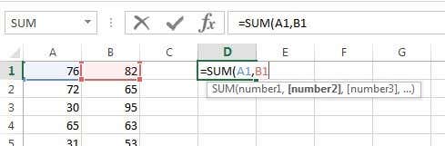
There are a couple of things to note while typing a formula in Excel. Firstly, you’ll notice that when you type the first opening parenthesis ( after the function name, Excel will automatically tell you what arguments that function takes. In our example, it shows number1, number2, etc. You separate arguments with commas. This particular function can take an infinite number of values since that is how the SUM function works.
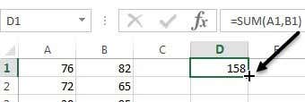
Secondly, either you can type in the cell reference manually (A1) or you can click on the cell A1 after you typed the open parenthesis. Excel will also highlight the cell in the same color as the cell reference so you can see the corresponding values exactly. So we summed one row together, but how can we sum all the other rows without typing the formula again or copying and pasting? Luckily, Excel makes this easy.
Move your mouse cursor to the bottom right corner of cell D1 and you’ll notice it changes from a white cross to a black plus sign.
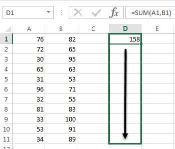
Now click and hold your mouse button down. Drag the cursor down to the last row with the data and then let go at the end.
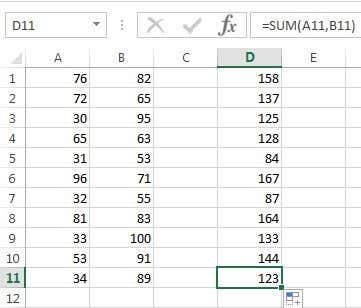
Excel is smart enough to know that the formula should change and reflect the values in the other rows rather than just showing you the same A1 + B1 all the way down. Instead, you’ll see A2+B2, A3+B3 and so on.
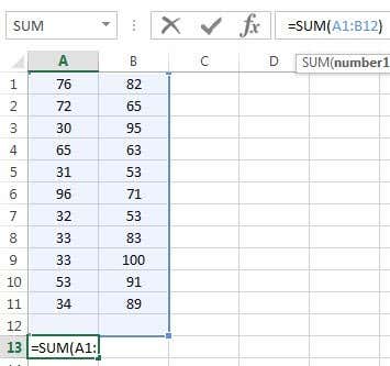
There is also another way to use SUM that explains another concept behind arguments in Excel. Let’s say we wanted to sum up all the values from A1 to A12, then how would we go about it? We could type something like =SUM(A1, A2, A3, etc), but that is very time consuming. A better way is to use an Excel range.
To sum A1 to A12, all we have to do is type =SUM(A1:A12) with a colon separating the two cell references instead of a comma. You could even type something like =SUM(A1:B12) and it will sum all values in A1 thru A12 and B1 thru B12.
This was a very basic overview of how to use functions and formulas in Excel, but it’s enough so that you can start using all of the data summation functions.
Summary Functions
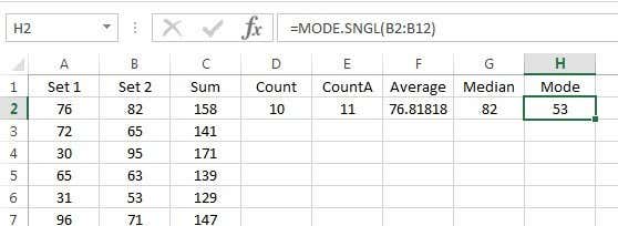
Using the same set of data, we’re going to use the rest of the summary functions to see what kind of numbers we can calculate. Let’s start with the COUNT and COUNTA functions.

Here I have entered the COUNT function into D2 and the COUNTA function into E2, using A2:A12 range as the data set for both functions. I also changed the value in A9 to the text string hello to show the difference. COUNT only counts the cells that have numbers whereas COUNTA counts cells that contain text and numbers. Both functions do not count blank cells. If you want to count blank cells, use the COUNTBLANK function.
Next up are the AVERAGE, MEDIAN and MODE functions. Average is self-explanatory, median is the middle number in a set of numbers and mode is the most common number or numbers in a set of numbers. In newer versions of Excel, you have MODE.SNGL and MODE.MULT because there could be more than one number that is the most common number in a set of numbers. I used B2:B12 for the range in the example below.
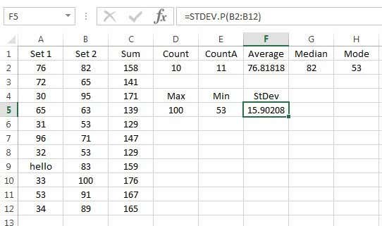
Moving on, we can calculate the MIN, MAX and STDEV for the set of numbers B2:B12. The STDEV function will calculate how widely values are dispersed from the average value. In newer versions of Excel, you have STDEV.P and STDEV.S, which calculates based on the entire population or based on a sample, respectively.
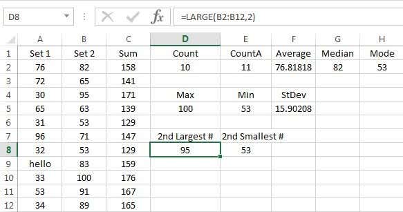
Finally, another two useful functions are LARGE and SMALL. They take two arguments: the cell range and the k-th largest value you want to return. So if you want the second largest value in the set, you would use 2 for the second argument, 3 for the third largest number, etc. SMALL works the same way, but gives you the k-th smallest number.
Lastly, there is a function called AGGREGATE, which allows you to apply any of the other functions mentioned above, but also lets you do things like ignore hidden rows, ignore error values, etc. You probably won’t need to use it that often, but you can learn more about it here in case you do need it.
So that’s a basic overview of some of the most common summary functions in Excel. If you have any questions, feel free to post a comment. Enjoy!
Founder of Online Tech Tips and managing editor. He began blogging in 2007 and quit his job in 2010 to blog full-time. He has over 15 years of industry experience in IT and holds several technical certifications. Read Aseem's Full Bio
Did you enjoy this tip? If so, check out our very own YouTube channel where we cover Windows, Mac, software, and apps, and have a bunch of troubleshooting tips and how-to videos. Click the button below to subscribe!

SUMIFS like other …IF or …IFS function are great tools to aggregate data based on a set of conditions. The downside of this approach is that the criteria must be supplied manually, especially when you need to create a summary table. In this guide, we’re going to show you how to use UNIQUE and SUMIFS functions in combination to generate an Excel summary table.
A summary table should include a unique list of categories. Creating a unique list of categories can become tedious as you keep adding more items in the future. To keep things simple and automate this task, you essentially can use either one of the two methods: Pivot Table or Excel formulas. Let's take a look at both.
Formula approach
Although Excel has a built-in feature for creating unique lists (or rather removing duplicate values), this actually requires a more manual approach. There were no dedicated formulas or tools since 2018 for creating a unique list of values. Traditionally, you had to use complex formulas to get a list of unique items.
Fortunately, Microsoft has introduced the UNIQUE formula in the later versions, which makes things much easier and automates most of this process. All you need is to do is to supply the reference of categories in your data. Excel will populate the unique list of values automatically.


Unfortunately, the UNIQUE function is available for Office 365 subscribers only at this time of article is written.
Pivot Table Approach
An alternative way to creating an Excel summary table is using a PivotTable. A PivotTable automatically creates a unique list of category items and aggregates the data. The approach is simple:
Читайте также: