
Xlfn excel что это

Despite how amazing Excel is there are times when you’ll find yourself shaking with fear! For example, have you ever seen anything as scary as this =ISERROR(FIND(_xlfn.CONCAT($A2:$E2),_xlfn.CONCAT($I$2:$M$6))) What is xlfn .
What’s The Story?
You open your friend’s Excel file and discover that some of the formulas aren’t working and include the letters XLFN ! You call your friend but he says that everything looks perfectly fine on his laptop. Did you get too much sun? Did you eat some bad fish? Did you smoke one of Oz du Soleil’s cigars?
What Is XLFN?
xlfn is a prefix added to functions that don’t exist in the version of Excel that you are using.
You have Excel 2013 and your friend has a newer version of Excel (Office 365 or Excel 2016). He uses a cool new function and sends the file to you. As you have Excel 2013 this cool new function doesn’t yet exist and you see xlfn in front of the function.
Recent XLFN Example
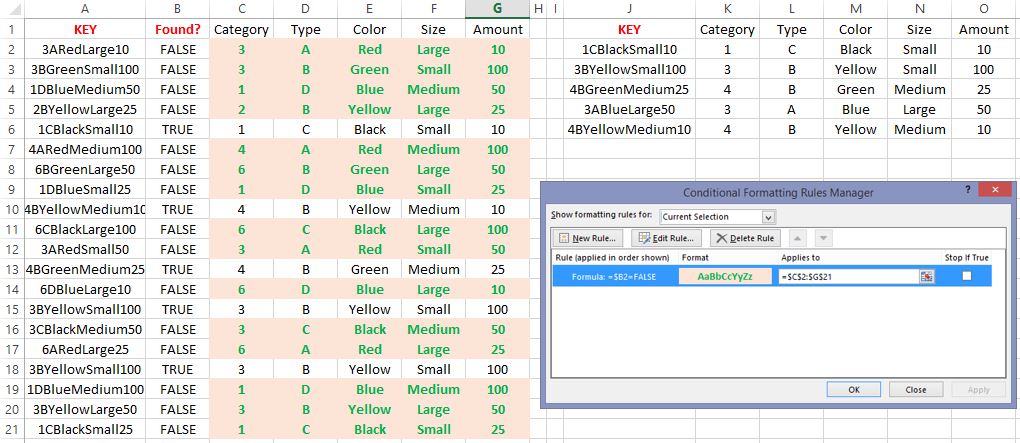
Last year I discovered David Hager’s Excel blog. He shares a lot of neat ideas. I recently saw this post: Conditional Format Rows in List 1 that are Not in List 2
When I opened the file I noticed that the solution wasn’t working for me. I went back to David’s post and looked at this pic:

I noticed that David used the CONCAT function. This must be a new Excel 2016 (or Office365?) function! There are a bunch of really interesting new functions but I’m still using Excel 2013.
What Does Microsoft Recommend?
“Remove the unsupported functions, or if possible, replace the unsupported functions with supported functions.” Also, read this .
OK. So, Is There A Workaround?
Although not as easy as David’s solution we can still produce the same end result.
Here are the steps to my workaround solution:
- Use a helper formula to concatenate all values in both tables: (i.e. =K2&L2&M2&N2&O2 )
- Adding this =ISNUMBER(MATCH(A2,$J$2:$J$6,0)) shows whether or not the row is found (Cell A2 is key in table 1. Column J is key in table 2)
- Add this formula inside your conditional formatting rule: =$B2=FALSE
Excel 2013 Workaround Solution
Here is David’s Excel file that includes my workaround solution for those that don’t have Excel 2016.
Learn From Excel MVP David Hager
About Me

My name is Kevin Lehrbass. I live in Markham, Ontario, Canada. I’ve been studying, supporting, building, troubleshooting, teaching and dreaming in Excel since 2001. I’m a Data Analyst.
There are so many amazing things that you can do with Excel.
Check out my recommended Excel Training section.
Check out my videos and my blog posts .
Away from Excel I enjoy learning Spanish, playing Chess, hanging out with Cali and Fenton and reading Excel books 🙂
ABOUT THE AUTHOR
Kevin Lehrbass
5 Comments → I SEE “XLFN” . WHAT IS HAPPENING?
How about Microsoft make the stand alone version of Office 2016 match the Office 365 version of Excel!
This can also happen when you have teammates working in a different language Excel than you. the xlfn, acts just like a flag that your local Excel creates to indicate that it tried looking for that formula but didn’t find it.
I don’t really know who on Ms decided that formulas in Excel should be translated and not ported between languages when you open the workbook, most surely in an effort to increase end-user retention of the formulae.
BITRSHIFT is another function from older versions of excel. It’s available in LibreOffice Calc.
Edit: should be “missing from older versions”
Huh you can also just use replace _xlfn.CONCAT to CONCATENATE
Leave a Reply Cancel reply
Sometimes I write a practical 'how to' post and other times I explore a crazy idea and build something unique. I love working with data in Microsoft Excel!
Kevin Lehrbass


= Мир MS Excel/Имена и макрос - Мир MS Excel
Войти через uID
Войти через uID
[/vba]
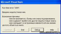
вываливается ошибка.
Причем вручную эти имена удаляются без проблем.
[/vba]
вываливается ошибка.
Причем вручную эти имена удаляются без проблем. RAN
[/vba]
вываливается ошибка.
Причем вручную эти имена удаляются без проблем. Автор - RAN
Дата добавления - 03.11.2013 в 11:35
Точно имена? Это ведь так 2003 и ниже воспринимает функции ЕСЛИОШИБКА и СУММЕСЛИМН Автор - Serge_007
Дата добавления - 03.11.2013 в 12:06
PS Обижаешь, начальник!
PS Обижаешь, начальник! RAN
Быть или не быть, вот в чем загвоздка!
PS Обижаешь, начальник! Автор - RAN
Дата добавления - 03.11.2013 в 12:12
[/vba]
(в текущий момент под рукой - версия 2003 с конвертером) Автор - ikki
Дата добавления - 03.11.2013 в 12:29
именно на Delete ошибка?
или на Debug.Print nm.Name после Delete?
пс. я знаю, что вопрос глупый, но вдруг.
именно на Delete ошибка?
или на Debug.Print nm.Name после Delete?
пс. я знаю, что вопрос глупый, но вдруг. ikki
пс. я знаю, что вопрос глупый, но вдруг. Автор - ikki
Дата добавления - 03.11.2013 в 12:47
Sub aa()
Dim nmm As Names
Set nmm = ThisWorkbook.Names
For i = 1 To nmm.Count
nmm(i).Delete
'Debug.Print nmm(i).Name
Next
End Sub
Писать - пишет, а удалять не хочет.
Sub aa()
Dim nmm As Names
Set nmm = ThisWorkbook.Names
For i = 1 To nmm.Count
nmm(i).Delete
'Debug.Print nmm(i).Name
Next
End Sub
Писать - пишет, а удалять не хочет. RAN
Sub aa()
Dim nmm As Names
Set nmm = ThisWorkbook.Names
For i = 1 To nmm.Count
nmm(i).Delete
'Debug.Print nmm(i).Name
Next
End Sub
Писать - пишет, а удалять не хочет. Автор - RAN
Дата добавления - 03.11.2013 в 12:53
кстати, удалять лучше в цикле For i = nmm.Count To 1 Step -1
но, конечно, проблема не в этом.
наверное, младшие Excel'и что-то добавили в свойства имён.
или неявно где-то используют такие имена.
на 2003-м не проверишь.
кстати, удалять лучше в цикле For i = nmm.Count To 1 Step -1
но, конечно, проблема не в этом.
наверное, младшие Excel'и что-то добавили в свойства имён.
или неявно где-то используют такие имена.
на 2003-м не проверишь.
ikki
В начале 2016 года Microsoft Excel выпустил очередной релиз своей программы. В этой заметке рассмотрены две новые текстовые функции Excel. На момент написания этой статьи они доступны пока только в режиме Excel online, поэтому скриншоты и последующий ролик записаны именно там.
Чтобы объединить содержимое нескольких ячеек в одну, традиционно используют формулу Excel СЦЕПИТЬ либо специальный оператор амперсанд &. В то же время у этой функции есть ряд недостатков. Основной из них — это необходимость каждую склеиваемую ячейку указывать в виде отдельного аргумента. При большом количестве склеиваемых ячеек приходится изрядно помучиться. С появлением новых функций СЦЕП и ОБЪЕДИНИТЬ этому неудобству пришел конец.
На смену СЦЕПИТЬ пришла функция СЦЕП, которая может сцепить целый диапазон! Теперь вместо отдельных ячеек A1;A2;A3;A4;A5;A6;A7;A8;A9;A10 достаточно указать диапазон A1:A10. Многие давно этого ждали. Дождались!

Однако радость кажется неполной, т.к. между словами обычно вставляют пробелы, запятые или какие-либо другие разделители, а СЦЕП этого не умеет. В примере выше нужно их либо сразу указать в конце каждого слова, либо опять же прописывать вручную. Вот бы здорово еще и разделители сами вставлялись.
Вы не поверите, но это как раз то, что умеет делать вторая текстовая функция эксель, о которой я хотел рассказать! Встречайте — ОБЪЕДИНИТЬ.
Ее синтаксис следующий.
ОБЪЕДИНИТЬ(разделитель; игнорировать_пустые; текст1; [текст2]; …)
разделитель – то, что должно вставляться между ячейками.
игнорировать_пустые – здесь ставится либо 0 (ЛОЖЬ), либо 1 (ИСТИНА). Если поставить 1, то пустые ячейки будут игнорироваться и разделители не будут дублироваться.
текст1; [текст2]; … – это либо отдельные ячейки, либо целый соединяемый диапазон.
В нашем примере функция ОБЪЕДИНИТЬ позволяет получить следующий результат.

Примечание. Некоторое время функция имела названия TEXTJOIN.
Я специально удалил бананы, чтобы показать отсутствие лишнего пробела после яблок.
Теперь объединить ячейки Excel, добавив к ним разделитель, можно всего за несколько секунд. Отличная функция ОБЪЕДИНИТЬ. Выглядит настолько круто, что хочется разработчикам пожать руку.
Подсчет максимального и минимального значения выполняется известными функциями МАКС и МИН. Бывает, что вычисления нужно произвести по группам или в зависимости от условия, как в СУММЕСЛИ.
Долгое время в Excel не было аналога СУММЕСЛИ или СРЗНАЧЕСЛИ для расчета максимального и минимального значения, поэтому использовали формулу массивов.
Пусть имеются данные
Нужно подсчитать максимальное значение в указанной группе. Название группы (критерий) введем в отдельную ячейку (D2). Пусть для начала это будет группа Б. Рядом введем следующую формулу:
Это формула массивов, поэтому ввести ее нужно комбинацией Ctrl + Shift + Enter.

Теперь, меняя название группы, можно без всяких фильтров и сводных таблиц видеть максимальное значение внутри этой группы.
Как это работает? Очень просто. Первым делом нужно указать диапазон, который будет использоваться в качестве аргумента функции МАКС, то есть только те ячейки, которые соответствуют указанной группе. Так как мы заранее позаботились об удобстве использования функции, то название группы указали не внутри формулы, а в отдельной ячейке (гораздо легче менять группу). Тогда формула для нужного диапазона выглядит так.
Указанное выражение отбирает только те значения, для которых название группы совпадает с условием в ячейке D2. Вот, как это видит Excel

На следующем этапе укажем функцию МАКС, аргументом которой выступает полученный выше массив. Excel воспринимает примерно так.

Видно, что максимальное значение внутри массива равно 31. Его и мы и увидим в ячейке с формулой. Нужно только не забыть итоговую функцию ввести комбинацией клавиш Ctrl + Shift + Enter, иначе ничего не получится. В строке формул формула массива отображается внутри фигурных скобок. Добавляются сами, специально дорисовывать не нужно.
Если функцию МАКС заменить на МИН, то по указанному условию (названию группы) будет выдаваться минимальное значение.
Функции Excel 2016 МАКСЕСЛИ (MAXIFS) и МИНЕСЛИ (MINIFS)
В MS Excel добавили новые статистические функции — МАКСЕСЛИ и МИНЕСЛИ. Обе функции имеют возможность учитывать несколько условий и некоторое время в их названиях в конце были буквы -МН. Потом убрали, хотя в скриншотах ниже используется вариант названий с -МН.
Есть ряд значений, каждое из которых входит в некоторую группу. Нужно рассчитать максимальное значение по группе А. Используем формулу МАКСЕСЛИ.

Все очень просто. Как и у СУММЕСЛИМН вначале указываем диапазон, где находится искомое максимальное значение (колонка В), затем диапазон с критериями (колонка А) и далее сам критерий (в ячейке D2). Можно указать сразу несколько условий. Таким же способом легко рассчитать минимальное значение по условию. Найдем, к примеру, минимум внутри группы Б.

Ниже показан ролик, как рассчитать максимальное и минимальное значение по условию.
In general a formula in Excel can be used directly in the write_formula() method:

However, there are a few potential issues and differences that the user should be aware of. These are explained in the following sections.
Non US Excel functions and syntax
Excel stores formulas in the format of the US English version, regardless of the language or locale of the end-user’s version of Excel. Therefore all formula function names written using XlsxWriter must be in English:
Also, formulas must be written with the US style separator/range operator which is a comma (not semi-colon). Therefore a formula with multiple values should be written as follows:
If you have a non-English version of Excel you can use the following multi-lingual formula translator to help you convert the formula. It can also replace semi-colons with commas.
Formula Results
XlsxWriter doesn’t calculate the result of a formula and instead stores the value 0 as the formula result. It then sets a global flag in the XLSX file to say that all formulas and functions should be recalculated when the file is opened.
This is the method recommended in the Excel documentation and in general it works fine with spreadsheet applications. However, applications that don’t have a facility to calculate formulas will only display the 0 results. Examples of such applications are Excel Viewer, PDF Converters, and some mobile device applications.
If required, it is also possible to specify the calculated result of the formula using the optional value parameter for write_formula() :
The value parameter can be a number, a string, a bool or one of the following Excel error codes:
It is also possible to specify the calculated result of an array formula created with write_array_formula() :
However, using this parameter only writes a single value to the upper left cell in the result array. For a multi-cell array formula where the results are required, the other result values can be specified by using write_number() to write to the appropriate cell:
Dynamic Array support
- FILTER()
- UNIQUE()
- SORT()
- SORTBY()
- XLOOKUP()
- XMATCH()
- RANDARRAY()
- SEQUENCE()
The following special case functions were also added with Dynamic Arrays:
Dynamic arrays are ranges of return values that can change in size based on the results. For example, a function such as FILTER() returns an array of values that can vary in size depending on the the filter results. This is shown in the snippet below from Example: Dynamic array formulas :
Which gives the results shown in the image below. The dynamic range here is “F2:I5” but it could be different based on the filter criteria.

It is also possible to get dynamic array behavior with older Excel functions. For example, the Excel function =LEN(A1) applies to a single cell and returns a single value but it is also possible to apply it to a range of cells and return a range of values using an array formula like . This type of “static” array behavior is called a CSE (Ctrl+Shift+Enter) formula. With the introduction of dynamic arrays in Excel 365 you can now write this function as =LEN(A1:A3) and get a dynamic range of return values. In XlsxWriter you can use the write_array_formula() worksheet method to get a static/CSE range and write_dynamic_array_formula() to get a dynamic range. For example:
Which gives the following result:

The difference between the two types of array functions is explained in the Microsoft documentation on Dynamic array formulas vs. legacy CSE array formulas. Note the use of the word “legacy” here. This, and the documentation itself, is a clear indication of the future importance of dynamic arrays in Excel.
For a wider and more general introduction to dynamic arrays see the following: Dynamic array formulas in Excel.
Dynamic Arrays - The Implicit Intersection Operator “@”
The Implicit Intersection Operator, “@”, is used by Excel 365 to indicate a position in a formula that is implicitly returning a single value when a range or an array could be returned.
We can see how this operator works in practice by considering the formula we used in the last section: =LEN(A1:A3) . In Excel versions without support for dynamic arrays, i.e. prior to Excel 365, this formula would operate on a single value from the input range and return a single value, like this:

There is an implicit conversion here of the range of input values, “A1:A3”, to a single value “A1”. Since this was the default behavior of older versions of Excel this conversion isn’t highlighted in any way. But if you open the same file in Excel 365 it will appear as follows:

The result of the formula is the same (this is important to note) and it still operates on, and returns, a single value. However the formula now contains a “@” operator to show that it is implicitly using a single value from the given range.
Finally, if you entered this formula in Excel 365, or with write_dynamic_array_formula() in XlsxWriter, it would operate on the entire range and return an array of values:
If you are encountering the Implicit Intersection Operator “@” for the first time then it is probably from a point of view of “why is Excel/XlsxWriter putting @s in my formulas”. In practical terms if you encounter this operator, and you don’t intend it to be there, then you should probably write the formula as a CSE or dynamic array function using write_array_formula() or write_dynamic_array_formula() (see the previous section on Dynamic Array support ).
A full explanation of this operator is shown in the Microsoft documentation on the Implicit intersection operator: @.
One important thing to note is that the “@” operator isn’t stored with the formula. It is just displayed by Excel 365 when reading “legacy” formulas. However, it is possible to write it to a formula, if necessary, using SINGLE() or _xlfn.SINGLE() . The unusual cases where this may be necessary are shown in the linked document in the previous paragraph.
In the section above on Dynamic Array support we saw that dynamic array formulas can return variable sized ranges of results. The Excel documentation refers to this as a “Spilled” range/array from the idea that the results spill into the required number of cells. This is explained in the Microsoft documentation on Dynamic array formulas and spilled array behavior.

Unfortunately, Excel doesn’t store the formula like this and in XlsxWriter you need to use the explicit function ANCHORARRAY() to refer to a spilled range. The example in the image above was generated using the following:
The Excel 365 LAMBDA() function
Note: at the time of writing the LAMBDA() function in Excel is only available to Excel 365 users subscribed to the Beta Channel updates.
Beta Channel versions of Excel 365 have introduced a powerful new function/feature called LAMBDA() . This is similar to the lambda function in Python (and other languages).
Consider the following Excel example which converts the variable temp from Fahrenheit to Celsius:
This could be called in Excel with an argument:
Or assigned to a defined name and called as a user defined function:
This is similar to this example in Python:
A XlsxWriter program that replicates the Excel is shown in Example: Excel 365 LAMBDA() function .
The formula is written as follows:
Note, that the parameters in the LAMBDA() function must have a “_xlpm.” prefix for compatibility with how the formulas are stored in Excel. These prefixes won’t show up in the formula, as shown in the image.

The LET() function is often used in conjunction with LAMBDA() to assign names to calculation results.
Formulas added in Excel 2010 and later
Excel 2010 and later added functions which weren’t defined in the original file specification. These functions are referred to by Microsoft as future functions. Examples of these functions are ACOT , CHISQ.DIST.RT , CONFIDENCE.NORM , STDEV.P , STDEV.S and WORKDAY.INTL .
When written using write_formula() these functions need to be fully qualified with a _xlfn. (or other) prefix as they are shown the list below. For example:
These functions will appear without the prefix in Excel:

Alternatively, you can enable the use_future_functions option in the Workbook() constructor, which will add the prefix as required:
If the formula already contains a _xlfn. prefix, on any function, then the formula will be ignored and won’t be expanded any further.
Enabling the use_future_functions option adds an overhead to all formula processing in XlsxWriter. If your application has a lot of formulas or is performance sensitive then it is best to use the explicit _xlfn. prefix instead.
The dynamic array functions shown in the Dynamic Array support section above are also future functions:
- _xlfn.UNIQUE
- _xlfn.XMATCH
- _xlfn.XLOOKUP
- _xlfn.SORTBY
- _xlfn._xlws.SORT
- _xlfn._xlws.FILTER
- _xlfn.RANDARRAY
- _xlfn.SEQUENCE
- _xlfn.ANCHORARRAY
- _xlfn.SINGLE
- _xlfn.LAMBDA
However, since these functions are part of a powerful new feature in Excel, and likely to be very important to end users, they are converted automatically from their shorter version to the explicit future function version by XlsxWriter, even without the use_future_function option. If you need to override the automatic conversion you can use the explicit versions with the prefixes shown above.
Using Tables in Formulas
Worksheet tables can be added with XlsxWriter using the add_table() method:
By default tables are named Table1 , Table2 , etc., in the order that they are added. However it can also be set by the user using the name parameter:
When used in a formula a table name such as TableX should be referred to as TableX[] (like a Python list):
Dealing with formula errors
- Ensure the formula is valid in Excel by copying and pasting it into a cell. Note, this should be done in Excel and not other applications such as OpenOffice or LibreOffice since they may have slightly different syntax.
- Ensure the formula is using comma separators instead of semi-colons, see Non US Excel functions and syntax above.
- Ensure the formula is in English, see Non US Excel functions and syntax above.
- Ensure that the formula doesn’t contain an Excel 2010+ future function as listed above ( Formulas added in Excel 2010 and later ). If it does then ensure that the correct prefix is used.
- If the function loads in Excel but appears with one or more @ symbols added then it is probably an array function and should be written using write_array_formula() or write_dynamic_array_formula() (see the sections above on Dynamic Array support and Dynamic Arrays - The Implicit Intersection Operator “@” ).
The following shows how to do that using Linux unzip and libxml’s xmllint to format the XML for clarity:
Читайте также: