
Где в эксель freeze
The tutorial demonstrates quick ways to freeze panes in Excel. You will learn how to quickly lock header row or/and the first column. You will also see how to freeze several panes at a time to make Excel always show certain rows or/and columns when you scroll down or right. These tips work in all modern versions of Excel 365, 2021, 2019, 2016, 2013, 2010 and 2007.
As you probably know, the current versions of Excel allow using more than a million rows and over 16,000 columns per sheet. Hardly anyone will ever use them to the limit, but if your worksheet contains tens or hundreds of rows, the column headers in the top row disappear when you are scrolling down to view lower entries. The good news is that you can easily fix that inconvenience by freezing panes in Excel.
In Microsoft Excel terms, to freeze panes means to always show certain rows and/or columns at the top of a spreadsheet when scrolling. Bellow you will find the detailed steps that work in any for Excel version.
How to freeze rows in Excel
Typically, you would want to lock the first row to see the column headers when you scroll down the sheet. But sometimes your spreadsheet may contain important information in a few top rows and you may want to freeze them all. Below you will find the steps for both scenarios.
How to freeze top row (header row) in Excel

To always show the header row, just go to the View tab, and click Freeze Panes > Freeze Top Row. Yep, it's that simple : )

Microsoft Excel gives you a visual clue to identify a frozen row by a bit thicker and darker border below it:
- If you are working with Excel tables rather than ranges, you do not really need to lock the first row, because the table header always stays fixed at the top, no matter how many rows down you scroll in a table.
- If you are going to print out your table and want to repeat header rows on every page, you may find this tutorial helpful - How to print row and column headers of Excel.
How to lock multiple Excel rows
Do you want to freeze several rows in your spreadsheet? No problem, you can lock as many rows as you want, as long as you always start with the top row.
-
Start by selecting the row below the last row you want to freeze.

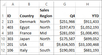
The result will be similar to what you see in the screenshot below - the top 2 rows in your Excel worksheet are frozen and will always show up.
Note. If some of the rows that you wish to lock are out of view when you apply freezing, they won't show up later, nor will you be able to scroll up to those rows. See how to avoid frozen hidden rows in Excel.
How to freeze columns in Excel
You lock columns in Excel in exactly the same way as you lock rows. And again, you can choose to freeze the first column only or multiple columns.
Lock the first column in a worksheet

Freezing the first column is as simple as clicking View > Freeze Panes > Freeze First Column.

A little darker and thicker border to the right of column A means that the left-most column in the table is frozen.
How to freeze multiple columns in Excel
If you want to lock more than one column in a sheet, proceed in this way:
-
Select the column to the right of the last column you want to freeze. For example, if you want to freeze the first 3 columns (A - C), select the entire column D or cell D1.
Note. Please make sure that all the columns you want to lock are visible at the moment of freezing. If some of the columns are out of view, you won't see them later. For more details, please see How to avoid hidden columns in Excel.
How to freeze multiple panes in Excel (rows and columns)
Do you wish to lock multiple rows and columns? No problem, you can do this as well, provided that you always start with the top row and first column.
To lock several rows and columns at a time, select a cell below the last row and to the right of the last column you want to freeze.

For example, to freeze the top row and first column , select cell B2, go to the View tab and click Freeze Panes under Freeze Panes:
In the same fashion, you can freeze as many Excel panes as you want. For instance, to lock the first 2 rows and 2 columns, you select cell C3; to fix 3 rows and 3 columns, select cell D4 etc. Naturally, the number of locked rows and columns does not necessarily have to be the same. For example, to freeze 2 rows and 3 columns, you select. guess which cell? Right, D3 : )
How to unfreeze panes in Excel
To unfreeze panes, just do the following: go to the View tab, Window group, and click Freeze panes > Unfreeze Panes.

Excel Freeze Panes tips
As you have just seen, freezing panes in Excel is one of the easiest tasks to perform. However, as is often the case with Microsoft, there is much more beneath the hood. What follows below is a caveat, an artifact and a tip.
Caveat: Prevent hidden rows / columns when freezing Excel panes
When you are locking several rows or columns in a spreadsheet, you may inadvertently hide some of them, and as a result, you won't see those hidden panes later. To avoid this, make sure that all the rows and/or columns you want to lock are within eyesight at the moment of freezing.

For example, you wish to freeze the first three rows, but row 1 is currently out of view, as shown in the screenshot below. As the result, row 1 won't show up later and you won't be able to scroll up to it. Though, you would still be able to get to the cells in a hidden frozen row using the arrow keys.
Artifact: Excel may freeze panes totally different from what you expected
Don't you believe me? Then try selecting cell A1, or the top visible row, or the leftmost visible column, click Freeze Panes and see what happens.

For example, if you select row 4 while the first 3 rows are out of view (not hidden, just above the scroll) and click Freeze Panes, what would you expect? Most obviously, rows 1 - 3 would get frozen? Nope! Microsoft Excel thinks differently and the screenshot below shows one of many possible outcomes:
So, please remember, the panes you are going to lock, both rows and columns, should always be in sight.
Tip: How to camouflage the Freeze Panes line

If you are not particularly fond of the dark freeze panes line that Microsoft Excel draws underneath locked rows and to the right of locked columns, you can try disguising it with the help of shapes and a little creativity : )
If you think this is something that might work for you, please see the following article for step-by-step instructions - Dealing with Excel Freeze Panes Line.
And this is all for today, thank you for reading!
You may also be interested in
62 comments to "How to freeze panes in Excel to lock rows and columns"
In your article: Artifact: Excel may freeze panes totally different from what you expected
I set up a worksheet open event: application.scrolltorow = 475, then do a activesheet.freezepanes=true: Resulted in freeze at row 475, ---but also freeze at row 501 and column "L".
In your illustration above, Excel had count down 25 rows and to the right 12 columns, they behaving exactly like mine ( 25 rows down and 12 columns to right)
Is this a bug in Excel? How we correct it,
Freeze panes is grayed out, un-useable. I've tried resaving my excel document, hoping that would cure it, but it is still grayed out and un-useable. No options give from the drop-down.
Office 365 is a great downgrade from my Office 97 that I use at home. I have other, most of the more recent versions on disk, but I choose user friendly over Microsoft Geek friendly.
Thank you for keeping it simple and easily to follow. So nice to find a web site that is too the point. :)
thank you very much. this information was very useful
We want to use more freeze pen in pivot table like in group one group finish then second group want to stop heading of the group name is it possible
how can we freeze column and row in same sheet on our choice not first row nor first column i want to do freeze 3rd row and 4th column in on sheet. please help to do that i waiting your answers. tayyab mirza from pakistan.
hello, please advise me how to convert DAYS:HOURS:MINUTES to total number of days.
eg. I have (2/22/16 11:00) in one cell and 3/15/16 20:00
in another cell, and the exact day difference is 22.375 days. Can you tell a quick formula for calculating this day difference in EXCEL SHEET. I SHALL BE VERY VERY GLAD FOR YOUR KIND SUPPORT. PLEASE.
THANKS, I AM AWAITING YOUR REPLY
I have seen spreadsheets where different rows are frozen
e.g.: The "title" (rows 1:3), followed by sub-titles for individual tables on the same page (row 6:7, 23:24, 41:42, 58:59, 74:75).
As you scroll down the page, the sheet allows you to scroll to each title then title automatically freezes and the page continues to scroll.
In the end, you can see all of the frozen titles/rows, and can continue scrolling to infinity.
How do you achieve this?
You want to scroll, but you want to see your top row or left column to stay still. To do this, you use the Freeze buttons on the View tab. If the Freeze buttons aren't available on the View tab, make sure you switch to Normal view. On the View tab, click Normal.
Freeze the top row
On the View tab, click Freeze Top Row.

When you do this, the border under row 1 is a little darker than other borders, meaning that the row above it is frozen.
Freeze the first column
If you'd rather freeze the leftmost column instead, on the View tab, click Freeze First Column.

When you do this, the line to the right of column A is a little darker than the other lines, meaning that the column to its left is frozen.
Freeze the top row and the first column
To freeze the top row and the first column at the same time, click cell B2. Then, on the View tab, click Freeze Panes.
Freeze as many rows or columns as you want
Want to freeze multiple rows and/or columns? You can freeze as many as you want, as long as you always start with the top row and the first column. To freeze multiple rows (starting with row 1), select the row below the last row you want frozen and click Freeze Panes. To freeze multiple columns, select the column to the right of the last column you want frozen and click Freeze Panes.
Say you want to freeze the top four rows and leftmost three columns. You'd select cell D5, and then on the View tab, click Freeze Panes. Any time you freeze rows and columns, the border below the last frozen row and to the right of the last frozen column appears a little thicker (here, below row 4 and to the right of column C).
Unfreeze rows or columns
Want to unfreeze a row, column, or both? On the View tab, click Unfreeze Panes.
The tutorial shows how to freeze cells in Excel to keep them visible while you navigate to another area of the worksheet. Below you will find the detailed steps on how to lock a row or multiple rows, freeze one or more columns, or freeze column and row at once.
When working with large datasets in Excel, you may often want to lock certain rows or columns so that you can view their contents while scrolling to another area of the worksheet. This can be easily done by using the Freeze Panes command and a few other features of Excel.
How to freeze rows in Excel
Freezing rows in Excel is a few clicks thing. You just click View tab > Freeze Panes and choose one of the following options, depending on how many rows you wish to lock:
- Freeze Top Row - to lock the first row.
- Freeze Panes - to lock several rows.
The detailed guidelines follow below.
How to freeze top row in Excel
To lock top row in Excel, go to the View tab, Window group, and click Freeze Panes > Freeze Top Row.

This will lock the very first row in your worksheet so that it remains visible when you navigate through the rest of your worksheet.

You can determine that the top row is frozen by a grey line below it:
How to freeze multiple rows in Excel
In case you want to lock several rows (starting with row 1), carry out these steps:
- Select the row (or the first cell in the row) right below the last row you want to freeze.
- On the View tab, click Freeze Panes >Freeze Panes.

For example, to freeze top two rows in Excel, we select cell A3 or the entire row 3, and click Freeze Panes:
As the result, you'll be able to scroll through the sheet content while continuing to view the frozen cells in the first two rows:

- Microsoft Excel allows freezing only rows at the top of the spreadsheet. It is not possible to lock rows in the middle of the sheet.
- Make sure that all the rows to be locked are visible at the moment of freezing. If some of the rows are out of view, such rows will be hidden after freezing. For more information, please see How to avoid frozen hidden rows in Excel.
How to freeze columns in Excel
Freezing columns in Excel is done similarly by using the Freeze Panes commands.
How to lock the first column
To freeze the first column in a sheet, click View tab > Freeze Panes > Freeze First Column.

This will make the leftmost column visible at all times while you scroll to the right.
How to freeze multiple columns in Excel
In case you want to freeze more than one column, this is what you need to do:
- Select the column (or the first cell in the column) to the right of the last column you want to lock.
- Go to the View tab, and click Freeze Panes >Freeze Panes.

For example, to freeze the first two columns, select the whole column C or cell C1, and click Freeze Panes:

This will lock the first two columns in place, as indicated by the thicker and darker border, enabling you to view the cells in frozen columns as you move across the worksheet:
- You can only freeze columns on the left side of the sheet. Columns in the middle of the worksheet cannot be frozen.
- All the columns to be locked should be visible, any columns that are out of view will be hidden after freezing.
How to freeze rows and columns in Excel
Besides locking columns and rows separately, Microsoft Excel lets you freeze both rows and columns at the same time. Here's how:
- Select a cell below the last row and to the right of the last column you'd like to freeze.
- On the View tab, click Freeze Panes >Freeze Panes.
Yep, it's that easy :)

For example, to freeze top row and first column in a single step, select cell B2 and click Freeze Panes:

This way, the header row and leftmost column of your table will always be viewable as you scroll down and to the right:
In the same fashion, you can freeze as many rows and columns as you want as long as you start with the top row and leftmost column. For instance, to lock top row and the first 2 columns, you select cell C2; to freeze the first two rows and the first two columns, you select C3, and so on.
How to unlock rows and columns in Excel

To unlock frozen rows and/or columns, go to the View tab, Window group, and click Freeze Panes > Unfreeze Panes.
Freeze Panes not working
If the Freeze Panes button is disabled (greyed out) in your worksheet, most likely it's because of the following reasons:
- You are in cell editing mode, for example entering a formula or editing data in a cell. To exit cell editing mode, press the Enter or Esc key.
- Your worksheet is protected. Please remove the workbook protection first, and then freeze rows or columns.
Other ways to lock columns and rows in Excel
Apart from freezing panes, Microsoft Excel provides a few more ways to lock certain areas of a sheet.
Split panes instead of freezing panes
Another way to freeze cells in Excel is to split a worksheet area into several parts. The difference is as follows:
Freezing panes allows you to keep certain rows or/and columns visible when scrolling across the worksheet.

Splitting panes divides the Excel window into two or four areas that can be scrolled separately. When you scroll within one area, the cells in the other area(s) remain fixed.
To split Excel's window, select a cell below the row or to the right of the column where you want the split, and click the Split button on the View tab > Window group. To undo a split, click the Split button again.
Use tables to lock top row in Excel

If you'd like the header row to always stay fixed at the top while you scroll down, convert a range to a fully-functional Excel table:
The fastest way to create a table in Excel is by pressing the Ctl + T shortcut. For more information, please see How to make a table in Excel.
Print header rows on every page
That's how you can lock a row in Excel, freeze a column, or freeze both rows and columns at a time. I thank you for reading and hope to see you on our blog next week!

В таблицах с большим количеством столбцов довольно неудобно выполнять навигацию по документу, ведь если она в ширину выходит за границы плоскости экрана, для того чтобы посмотреть названия строк, в которые занесены данные, придется постоянно прокручивать страницу влево, а потом опять возвращаться вправо. На эти операции будет уходить дополнительное количество времени. Поэтому для того, чтобы пользователь мог экономить своё время и силы, в программе Microsoft Excel предусмотрена возможность закрепить столбцы. После выполнения данной процедуры левая часть таблицы, в которой находятся наименования строк, всегда будет на виду. Давайте же разберемся, как зафиксировать столбцы в приложении Excel.
Закрепление столбца в таблице Эксель
При работе с «широкой» таблицей может потребоваться закрепить как один, так и сразу несколько столбцов (область). Делается это буквально в несколько кликов, а непосредственный алгоритм выполнения в каждом из двух случаев отличается буквально на один пункт.
Вариант 1: Один столбец
Для того чтобы закрепить крайний левый столбец, можно даже не выделять его предварительно – программа сама поймет, для какого элемента таблицы требуется принять указанное вами изменение.


Вариант 2: Несколько столбцов (область)
Бывает и так, что закрепить требуется более одного столбца, то есть область таковых. В данном случае необходимо учесть всего один важный нюанс – не выделяйте диапазон столбцов.
- Выделите столбец, следующий за той областью, которую планируете закрепить. То есть, если требуется закрепить диапазон A-C, выделять необходимо D.
- Перейдите во вкладку «Вид».
- Кликните по меню «Закрепить области» и выберите в нем аналогичный пункт.
Открепление зафиксированной области
Если необходимость в закреплении столбца или столбцов отпала, во все той же вкладке «Вид» программы Эксель откройте меню кнопки «Закрепить области» и выберите вариант «Снять закрепление областей». Это сработает как для одного элемента, так и для диапазона таковых.

Заключение
Как видите, в табличном процессоре Microsoft Excel можно легко закрепить всего один, крайний левый столбец или диапазон таковых (область). Открепить их, если такая необходимость появится, тоже можно буквально в три клика.

Мы рады, что смогли помочь Вам в решении проблемы.
Отблагодарите автора, поделитесь статьей в социальных сетях.
Опишите, что у вас не получилось. Наши специалисты постараются ответить максимально быстро.
При работе с большими наборами данных в Excel вам может потребоваться заблокировать определенные строки или столбцы, чтобы вы могли видеть их содержимое при прокрутке в другую область рабочего листа. Ниже вы найдете подробные инструкции о том, как закрепить одну или несколько строк, зафиксировать один или несколько столбцов или «заморозить» и то, и другое одновременно, а также как снять блокировку. В Excel есть специальные инструменты, чтобы зафиксировать шапку таблицы, первые столбцы или же и то, и другое сразу.
Возможность закрепить строку — очень важный лайфхак в Экселе. Научившись этому простому приему, вы сможете просматривать любую область таблицы, не теряя из поля зрения строку с именами столбцов или так называемую «шапку» таблицы.
Это можно легко сделать с помощью меню Закрепить области и нескольких других функций.
Итак, как закрепить строку в Excel? Разберём самое важное:

«Замораживание» на экране части информации - это всего лишь несколько щелчков мышью. Вы просто нажимаете вкладку «Вид» > и выбираете один из параметров в зависимости от того, что вы хотите заблокировать (как на скриншоте ниже).
А теперь объясним подробнее.
Как закрепить верхнюю строку в Excel.
Если ваша таблица содержит большое количество строк, то при прокрутке вниз шапка с названиями колонок скроется из виду. И вам будет достаточно сложно ориентироваться в изобилии цифр. Ведь довольно сложно запомнить, что записано в каждом из столбцов. Или придется постоянно прокручивать таблицу вверх-вниз. Поэтому эту проблему нужно обязательно решить, закрепив одну или несколько верхних строк таблицы.
Рассмотрим, как зафиксировать строку в Excel при прокрутке таблицы вниз. Перейдите на вкладку «Вид» и действуйте так, как показано на рисунке.
Это действие заблокирует самую первую строку в вашем рабочем листе Excel, чтобы она оставалась на виду при навигации по данным.

Выбираем пункт "Закрепить верхнюю строку".
Вы можете визуально определить, что шапка таблицы «заморожена», видя серую линию под ней:

Закреплена первая строка
Как «заморозить» несколько строк.
Но очень часто бывает, что шапка таблицы расположена в нескольких верхних строках. Если вы хотите заблокировать несколько строчек (начиная с первой), то выполните следующие действия:
- Выберите строку (или просто первую позицию в ней), информацию выше которой вы хотите видеть постоянно. Например, если заголовки столбцов занимают первые две строки, то установите курсор в первую ячейку третьей строки.
- На вкладке «Вид» нажмите
Например, чтобы заблокировать две верхние строки на листе, мы выбираем ячейку A3 и выбираем первый пункт в меню:

Закрепляем область выше и левее курсора.
Как видно на скриншоте, если мы хотим зафиксировать первые две строчки, устанавливаем курсор на третью. В результате вы сможете прокручивать содержимое листа, а на экране всегда будет оставаться шапка таблицы.
Предупреждения:
- Учтите, что при закреплении области таблицы будут зафиксированы все строки и столбцы, которые находятся выше и левее указанной ячейки. Поэтому, если вы хотите закрепить только строки, то установите курсор в ячейку первого столбца перед использованием инструмента.
- Microsoft Excel при прокрутке таблицы позволяет замораживать только содержимое верхней части рабочего листа. Невозможно заблокировать что-либо в середине.
- Убедитесь, что все фиксируемые данные видны в момент «замораживания». Если какие-то данные не видны, то они будут скрыты.
- Если вы вставите строку перед той, что была закреплена (в нашем случае, между первой и второй), то она тоже будет зафиксирована.
Как зафиксировать столбец в Excel
Теперь рассмотрим, как закрепить столбец в Excel при прокрутке вправо. Эта операция выполняется аналогично рассмотренным выше действиям со строками.
Как заблокировать первый столбец.
Чтобы закрепить столбец при прокрутке вправо, выберите в выпадающем меню — «Закрепить первый столбец».
Это сделает первую слева колонку постоянно видимой во время горизонтальной прокрутки вправо.
Как «заморозить» несколько столбцов.
Чтобы зафиксировать более одного столбца, это то, что вам нужно сделать:
- Выберите столбец (или первую позицию в нем) справа от последнего столбца, который вы хотите заблокировать.
- Перейдите на вкладку «Вид» и нажмите
Например, чтобы заморозить первые два столбца, выделите всю колонку C или просто поставьте курсор в ячейку C1 и нажмите как на скриншоте:

Зафиксируем первые два столбца
Это позволит вам постоянно видеть первые 2 позиции с левой стороны при перемещении по рабочему листу.
Предупреждения:
- Вы можете закрепить столбец только слева, на краю вашей таблицы. Столбцы в середине таблицы не могут быть зафиксированы.
- Все столбцы, которые нужно заблокировать, должны быть видны. Все, которые не видны, будут скрыты после фиксации.
- Если вы вставите колонку перед той, что была закреплена, новая колонка будет также закрепленной. В нашем примере, если вы вставите столбец между A и B, то Excel при прокрутке зафиксирует уже 3 первых столбца.
Как закрепить строку и столбец одновременно.
Помимо блокировки по отдельности, Microsoft Excel позволяет замораживать одновременно ячейки по вертикали и горизонтали. Вот как делается закрепление областей :
- Выберите клетку ниже и справа от той области, которую вы хотите заблокировать. К примеру, если мы хотим постоянно видеть на экране шапку таблицы, состоящую из двух строчек, а также первые две колонки слева, то ставим курсор в C3.
- На вкладке «Вид» выберите .
Да, это так просто :)
Примечание. Фиксируется весь диапазон, который находится выше и левее курсора.
Таким же образом вы можете заморозить столько по вертикали и горизонтали, сколько захотите. Но при условии, что вы начинаете с верхнего ряда и самой левой колонки.
Например, чтобы заблокировать верхнюю строку и первые 2 столбика, вы выбираете C2; чтобы заморозить первые две строчки и первые две колонки, выберите C3 и т. д.
Обратите внимание, что, чтобы закрепить строку и столбец, действуют те же правила, о которых мы говорили выше. Зафиксировано будет только то, что видно на экране. Все, что находится выше и правее и не попадает на экран на момент совершения операции, будет просто скрыто.
Как разблокировать строки и столбцы?
Чтобы разблокировать «зафиксированные» данные, перейдите на вкладку «Вид» и нажмите «Снять закрепление …». Эта кнопка появляется в меню, только если вы закрепили какие-то строки либо столбцы.

При этом уже не важно, где расположен курсор и в каком месте листа вы находитесь.
Почему не работает?
Если кнопка отключена (выделена серым цветом) то, скорее всего, это происходит по следующим причинам:
- Вы находитесь в режиме редактирования. Например, происходит ввод формулы или редактирование данных. Чтобы выйти из режима редактирования, нажмите Enter или Esc.
- Ваш рабочий лист защищен. Пожалуйста, сначала снимите защиту рабочей книги, а затем действуйте, как описано выше в этой статье.
Другие способы закрепления столбцов и строк.
Еще один способ несколько нестандартный способ - это разделить экран на несколько частей. Особенность этого приёма заключается в следующем:
Разделение панелей делит ваш экран на две или же четыре области, которые можно просматривать независимо друг от друга. При прокрутке внутри одной из них ячейки в другой остаются на прежнем месте.

Чтобы разделить окно на части, выберите позицию снизу или справа от того места, в котором вы хотите это сделать, и нажмите соответствующую кнопку. Чтобы отменить операцию, снова нажмите её же.
Еще один способ - использование «умной» таблицы для блокировки её заголовка.
Если вы хотите, чтобы заголовок всегда оставался фиксированным вверху при прокрутке вниз, преобразуйте диапазон в таблицу Excel:

Самый быстрый способ создать таблицу в Excel - нажать Ctl + T.
Однако при этом учитывайте, что если шапка состоит более чем из 1 строчки, то зафиксируется только первая из них. В результате может получиться не очень красиво.
Печать заголовка таблицы на каждой странице
Если вы хотите повторить одну или несколько верхних строк листа Excel на каждой напечатанной странице, переключитесь на вкладку «Разметка страницы» и нажмите кнопку «Печатать заголовки». Далееперейдите на вкладку «Лист» и выберите сквозные строки.
Несколько советов и предупреждений.
Как вы только что видели, фиксация областей в Excel - одна из самых простых задач. Однако, как это часто бывает с Microsoft, внутри скрывается гораздо больше.
Предостережение: предотвращение полного исчезновения строк и столбцов при закреплении областей рабочей книги.
Когда вы блокируете несколько строк или столбцов в электронной таблице, вы можете непреднамеренно скрыть некоторые из них, и в результате потом вы уже не увидите их. Чтобы избежать этого, убедитесь, что всё, что вы хотите зафиксировать, находится в поле зрения в момент осуществления операции.
Например, вы хотите заморозить первые две строчки, но первая в настоящее время не видна, как показано на скриншоте ниже. В результате первая из них не будет отображаться позже, и вы не сможете переместиться на нее. Тем не менее, вы все равно сможете установить курсор в ячейку в скрытой замороженной позиции с помощью клавиш управления курсором (которые со стрелками) и при необходимости даже изменить её.

Excel может зафиксировать области несколько иначе, чем вы ожидали.
Вы мне не верите? Тогда попробуйте выбрать ячейку A3, когда первые две не видны (просто находятся чуть выше видимой части таблицы), и щелкните . Что вы ожидаете? Что строки 1 - 2 будут заморожены? Нет! Microsoft Excel думает иначе, и на снимке экрана ниже показан один из многих возможных результатов:

Неподвижной стали ¾ экрана. Вряд ли с такой логикой программы можно согласиться.
Поэтому, пожалуйста, помните, что данные, которые вы собираетесь зафиксировать, всегда должны быть полностью видны.
Совет: Как замаскировать линию, отделяющую закрепленную область.
Если вам не нравится тёмная линия, которую Microsoft Excel рисует внизу и справа от зафиксированной области, вы можете попытаться замаскировать ее с помощью шаблонов оформления и небольшого творческого подхода:)

Выберите приятный для вас вариант оформления нижней границы ячеек, и линия не будет раздражать вас.
Вот как вы можете заблокировать строку в Excel, зафиксировать столбец или одновременно сделать и то, и другое.
Читайте также: