
Data table excel как использовать
The tutorial shows how to use data tables for What-If analysis in Excel. Learn how to create a one-variable and two-variable table to see the effects of one or two input values on your formula, and how to set up a data table to evaluate multiple formulas at once.
You have built a complex formula dependent on multiple variables and want to know how changing those inputs changes the results. Instead of testing each variable individually, make a What-if analysis data table and observe all possible outcomes with a quick glance!
What is a data table in Excel?
In Microsoft Excel, a data table is one of the What-If Analysis tools that allows you to try out different input values for formulas and see how changes in those values affect the formulas output.
Data tables are especially useful when a formula depends on several values, and you'd like to experiment with different combinations of inputs and compare the results.
Currently, there exist one variable data table and two variable data table. Although limited to a maximum of two different input cells, a data table enables you to test as many variable values as you want.
Note. A data table isn't the same thing as an Excel table, which is purposed for managing a group of related data. If you are looking to learn about many possible ways to create, clear and format a regular Excel table, not data table, please check out this tutorial: How to make and use a table in Excel.
How to create a one variable data table in Excel
One variable data table in Excel allows testing a series of values for a single input cell and shows how those values influence the result of a related formula.
To help you better understand this feature, we are going to follow a specific example rather than describing generic steps.
- B8 contains the FV formula that calculates the closing balance.
- B2 is the variable you want to test (initial investment).

And now, let's do a simple What-If analysis to see what your savings will be in 5 years depending on the amount of your initial investment, ranging from $1,000 to $6,000.
Here are the steps to make a one-variable data table:

- Enter the variable values either in one column or across one row. In this example, we are going to create a column-oriented data table, so we type our variable values in a column (D3:D8) and leave at least one blank column to the right for the outcomes.
- Type your formula in the cell one row above and one cell to the right of the variable values (E2 in our case). Or, link this cell to the formula in your original dataset (if you decide to change the formula in the future, you would need to update only one cell). We choose the latter option, and enter this simple formula in E2: =B8
Tip. If you want to examine the impact of the variable values on other formulas that refer to the same input cell, enter the additional formula(s) to the right of the first formula, as shown in this example.

Now, you can take a quick look at your one-variable data table, examine the possible balances and choose the optimal deposit size:
Row-oriented data table
The above example shows how to set up a vertical, or column-oriented, data table in Excel. If you prefer a horizontal layout, here's what you need to do:

- Type the variable values in a row, leaving at least one empty column to the left (for the formula) and one empty row below (for the results). For this example, we enter the variable values in cells F3:J3.
- Enter the formula in the cell that is one column to the left of your first variable value and one cell below (E4 in our case).
- Make a data table as discussed above, but enter the input value (B3) in the Row input cell box:
How to make a two variable data table in Excel
A two-variable data table shows how various combinations of 2 sets of variable values affect the formula result. In other words, it shows how changing two input values of the same formula changes the output.
The steps to create a two-variable data table in Excel are basically the same as in the above example, except that you enter two ranges of possible input values, one in a row and another in a column.
To see how it works, let's use the same compound interest calculator and examine the effects of the size of the initial investment and the number of years on the balance. To have it done, set up your data table in this way:
- Enter your formula in a blank cell or link that cell to your original formula. Make sure you have enough empty columns to the right and empty rows below to accommodate your variable values. As before, we link the cell E2 to the original FV formula that calculates the balance: =B8
- Type one set of input values below the formula, in the same column (investment values in E3:E8).
- Enter the other set of variable values to the right of the formula, in the same row (number of years in F2:H2).
Data table to compare multiple results
If you wish to evaluate more than one formula at the same time, build your data table as shown in the previous examples, and enter the additional formula(s):
- To the right of the first formula in case of a vertical data table organized in columns
- Below the first formula in case of a horizontal data table organized in rows
For the "multi-formula" data table to work correctly, all the formulas should refer to the same input cell.
As an example, let's add one more formula to our one-variable data table to calculate the interest and see how it is affected by the size of the initial investment. Here's what we do:

Voilà, you can now observe the effects of your variable values on both formulas:
Data table in Excel - 3 things you should know
To effectively use data tables in Excel, please keep in mind these 3 simple facts:
- For a data table to be created successfully, the input cell(s) must be on the same sheet as the data table.
- Microsoft Excel uses the TABLE(row_input_cell, colum_input_cell) function to calculate data table results:
- In one-variable data table, one of the arguments is omitted, depending on the layout (column-oriented or row-oriented). For example, in our horizontal one-variable data table, the formula is =TABLE(, B3) where B3 is the column input cell.
- In two-variable data table, both arguments are in place. For example, =TABLE(B6, B3) where B6 is the row input cell and B3 is the column input cell.
How to delete a data table in Excel
As mentioned above, Excel does not allow deleting values in individual cells containing the results. Whenever you try to do this, an error message "Cannot change part of a data table" will show up.
However, you can easily clear the entire array of the resulting values. Here's how:
- Depending on your needs, select all the data table cells or only the cells with the results.
- Press the Delete key.
How to edit data table results
Since it is not possible to change part of an array in Excel, you cannot edit individual cells with calculated values. You can only replace all those values with your own one by performing these steps:
- Select all the resulting cells.
- Delete the TABLE formula in the formula bar.
- Type the desired value, and press Ctrl + Enter .

This will insert the same value in all the selected cells:
Once the TABLE formula is gone, the former data table becomes a usual range, and you are free to edit any individual cell normally.
How to recalculate data table manually
If a large data table with multiple variable values and formulas slows down your Excel, you can disable automatic recalculations in that and all other data tables.

For this, go to the Formulas tab > Calculation group, click the Calculation Options button, and then click Automatic Except Data Tables.
This will turn off automatic data table calculations and speed up recalculations of the entire workbook.
To manually recalculate your data table, select its resulting cells, i.e. the cells with TABLE() formulas, and press F9 .
This is how you create and use a data table in Excel. To have a closer look at the examples discussed this this tutorial, you are welcome to download our sample Excel Data Tables workbook. I thank you for reading and would be happy to see you again next week!
Таблица данных в Excel представляет собой диапазон, который оценивает изменение одной или двух переменных в формуле. Другими словами, это Анализ "что если", о котором мы говорили в одной из прошлых статей (если Вы ее не читали - очень рекомендую ознакомиться по этой ссылке), в удобном виде. Вы можете создать таблицу данных с одной или двумя переменными.
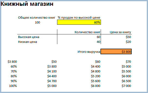
Предположим, что у Вас есть книжный магазин и в нем есть 100 книг на продажу. Вы можете продать определенный % книг по высокой цене - $50 и определенный % книг по более низкой цене - $20. Если Вы продаете 60% книг по высокой цене, в ячейке D10 вычисляется общая выручка по форуме 60 * $50 + 40 * $20 = $3800.
Таблица данных с одной переменной.
Что бы создать таблицу данных с одной переменной, выполните следующие действия:
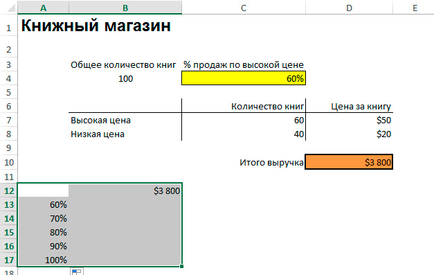
1. Выберите ячейку B12 и введите =D10 (ссылка на общую выручку).
2. Введите различные проценты в столбце А.
3. Выберите диапазон A12:B17.
Мы будет рассчитывать общую выручку, если Вы продаете 60% книг по высокой цене, 70% книг по высокой цене и т.д.
4. На вкладке Данные, кликните на Анализ "что если" и выберите Таблица данных из списка.

5. Кликните в поле "Подставлять значения по строкам в: "и выберите ячейку C4.

Мы выбрали ячейку С4 потому что проценты относятся к этой ячейке (% книг, проданных по высокой цене). Вместе с формулой в ячейке B12, Excel теперь знает, что он должен заменять значение в ячейке С4 с 60% для расчета общей выручки, на 70% и так далее.
Примечание: Так как мы создает таблицу данных с одной переменной, то вторую ячейку ввода ("Подставлять значения по столбцам в: ") мы оставляем пустой.
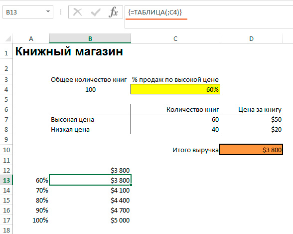
Вывод: Если Вы продадите 60% книг по высокой цене, то Вы получите общую выручку в размере $3 800, если Вы продадите 70% по высокой цене, то получите $4 100 и так далее.
Примечание: Строка формул показывает, что ячейки содержат формулу массива. Таким образом, Вы не можете удалить один результат. Что бы удалить результаты, выделите диапазон B13:B17 и нажмите Delete.
Таблица данных с двумя переменными.
Что бы создать таблицу с двумя переменными, выполните следующие шаги.
1. Выберите ячейку A12 и введите =D10 (ссылка на общую выручку).
2. Внесите различные варианты высокой цены в строку 12.
3. Введите различные проценты в столбце А.
4. Выберите диапазон A12:D17.
Мы будем рассчитывать выручку от реализации книг в различных комбинациях высокой цены и % продаж книг по высокой цене.

5. На вкладке Данные, кликните на Анализ "что если" и выберите Таблица данных из списка.

6. Кликните в поле "Подставлять значения по столбцам в: " и выберите ячейку D7.
7. Кликните в поле "Подставлять значения по строкам в: " и выберите ячейку C4.
Мы выбрали ячейку D7, потому что высокая цена на книги задается именно в этой ячейке. Мы выбрали ячейку C4, потому что процент продаж по высокой цене задается именно в этой ячейке. Вместе с формулой в ячейке A12, Excel теперь знает, что он должен заменять значение ячейки D7 начиная с $50 и в ячейке С4 начиная с 60% для расчета общей выручки, до $70 и 100% соответсвенно.


Вывод: Если Вы продадите 60% книг по высокой цене в размере $50, то Вы получите общую выручку $3 800, если Вы продадите 80% по высокой цене в размере $60, то получите $5 200 и так далее.
Примечание: строка формул показывает, что ячейки содержат формулу массива. Таким образом, вы не можете удалить один результат. Что бы удалить результаты, выделите диапазон B13:D17 и нажмите Delete.
Спасибо за внимание. Теперь Вы сможете более эффективно применять один из видов анализа "что если" , а именно формирование таблиц данных с одной или двумя переменными.
Остались вопросы - задавайте их в комментариях ниже, также не забывайте подписываться на нас в социальных сетях.
Сводная таблица в Excel является отличным инструментом для агрегирования и анализа данных. В Pandas есть подобный функционал под названием pivot_table, который мы сегодня разберемся как использовать.

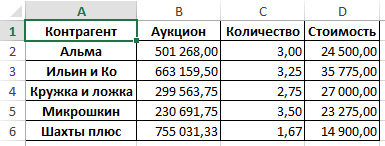
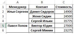
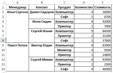
Для начала давайте представим, что мы являемся аналитиками в фирме по продаже компьютеров, программного обеспечения к ним, а также оказываем услуги по техническому сопровождению. Нам поставлена задача проанализировать участие компании в различных аукционах. Таблица с исходными данными представлена ниже:
| Аукцион | Контрагент | Контакт | Менеджер | Продукт | Количество | Цена | Статус |
| 424845 | Ильин и Ко | Сергей Ильин | Илья Сергеев | Компьютер | 4 | 45 200 | на рассмотрении |
| 312058 | Ильин и Ко | Сергей Ильин | Илья Сергеев | Софт | 2 | 37 600 | на рассмотрении |
| 918390 | Ильин и Ко | Сергей Ильин | Илья Сергеев | Тех. сопровождение | 2 | 21 200 | в ожидании |
| 997345 | Ильин и Ко | Сергей Ильин | Илья Сергеев | Компьютер | 5 | 39 100 | отменен |
| 496901 | Шахты плюс | Данил Сидоров | Илья Сергеев | Компьютер | 3 | 13 600 | выигран |
| 800437 | Шахты плюс | Данил Сидоров | Илья Сергеев | Компьютер | 1 | 24 400 | в ожидании |
| 967756 | Шахты плюс | Данил Сидоров | Илья Сергеев | Софт | 1 | 6 700 | на рассмотрении |
| 871434 | Альма | Женя Сидин | Илья Сергеев | Тех. сопровождение | 2 | 7 000 | в ожидании |
| 131102 | Альма | Женя Сидин | Илья Сергеев | Компьютер | 4 | 42 000 | отменен |
| 191777 | Микрошкин | Сергей Минин | Павел Попов | Компьютер | 3 | 28 900 | выигран |
| 225531 | Микрошкин | Сергей Минин | Павел Попов | Компьютер | 5 | 15 000 | на рассмотрении |
| 159172 | Микрошкин | Сергей Минин | Павел Попов | Тех. сопровождение | 2 | 2 300 | в ожидании |
| 346287 | Микрошкин | Сергей Минин | Павел Попов | Софт | 4 | 46 900 | на рассмотрении |
| 170247 | Кружка и ложка | Виктор Юдин | Павел Попов | Тех. сопровождение | 1 | 14 800 | выигран |
| 769790 | Кружка и ложка | Виктор Юдин | Павел Попов | Компьютер | 1 | 47 500 | выигран |
| 106612 | Кружка и ложка | Виктор Юдин | Павел Попов | Компьютер | 5 | 36 400 | отменен |
| 151606 | Кружка и ложка | Виктор Юдин | Павел Попов | Монитор | 4 | 9 300 | на рассмотрении |
Сохраните таблицу в Excel файл, вставив начиная с ячейки А1, а также назовите лист "База". Сохраните файл с названием "Отчет по аукционам.xlsx".
Итак сначала давайте прочитаем данные из Excel файла, создадим Pandas Dataframe и передадим туда данные:
import pandas as pd
import numpy as np
data_pd=pd.read_excel('Отчет по аукционам.xlsx',sheet_names='База')
Отлично, теперь давайте столбец "Статус" переведем в тип "category" для того, что бы в дальнейшем данные у нас были структурированы:
data_pd['Статус'] = data_pd['Статус'].astype('category')
data_pd['Статус'].cat.set_categories(['выигран','в ожидании','на рассмотрении','отменен'],inplace=True)
Выводить данные мы можем как в консоль Python, так и в Excel файл. Выберем второй вариант. Эта строка должна быть последней в коде, весь остальной код, который мы будем рассматривать ниже, должен располагаться перед этой строкой. Сохраните скрипт в туже папку, что и файл Отчет по аукционам.xlsx:
Сводная таблица в Python
Cоздать сводную таблицу в Python при помощи пакета Pandas очень просто. К примеру давайте создадим сводную таблицу по столбцу Контрагент:
data_pt = pd.pivot_table(data_pd,index=['Контрагент'])
Откройте файл result.xlsx, который скрипт создал в той же папке, где он располагается. Результат должен быть следующего вида:
Мы можем создать сводную таблицу по нескольким индексируемым столбцам:
data_pt = pd.pivot_table(data_pd,index=['Контрагент', 'Контакт', 'Менеджер'])

По умолчанию сводная таблица выводится по всем числовым полям, однако это не всегда удобно, а иногда и лишено смысла, поэтому можно выводить сводные данные только по отдельным столбцам. Для примера выведем только столбец "Стоимость", для этого добавим параметр values=['Стоимость']:
data_pt = pd.pivot_table(data_pd,index=['Менеджер', 'Контакт'], values=['Стоимость'])
Столбец стоимость по умолчанию выводит среднее значение, однако нам скорее интересна сумма продаж. Добавляем параметр aggfunc=np.sum:
data_pt = pd.pivot_table(data_pd,index=['Менеджер', 'Контакт'], values=['Стоимость'], aggfunc=np.sum)

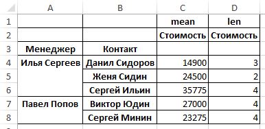
С помощью aggfunc можно выводить несколько значений, к примеру средную стоимость и количество продаж:
data_pt = pd.pivot_table(data_pd,index=['Менеджер', 'Контакт'], values=['Стоимость'], aggfunc=[np.mean,len])
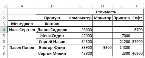
Также как в Excel, в Pandas индексируемые параметры можно выводить не только в строки, но и в столбцы, для этого служит параметр columns. Например выведем в столбцы наименование продуктов:
data_pt = pd.pivot_table(data_pd,index=['Менеджер', 'Контакт'], values=['Стоимость'], columns=['Продукт'], aggfunc=np.sum)
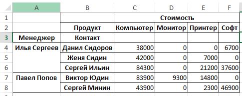
Наверное вы обратили внимание, что в ячейках, где нет данных пусто, хотя нам привычнее, что бы в таких полях указывалось бы значение 0. Добавим параметр fill_value=0:
data_pt = pd.pivot_table(data_pd,index=['Менеджер', 'Контакт'], values=['Стоимость'], columns=['Продукт'], aggfunc=np.sum ,fill_value=0)
Вероятно полезно было бы рассматривать эффективность деятельности наших менеджеров не только по стоимости продаж, но и по их количеству.
data_pt = pd.pivot_table(data_pd,index=['Менеджер', 'Контакт'], values=['Стоимость', 'Количество'], columns=['Продукт'], aggfunc=np.sum ,fill_value=0)

Как и в Excel, мы можем перемещать индексируемые поля между столбцами и строками. К примеру перенесем "Продукт" из столбцов в строки:
data_pt = pd.pivot_table(data_pd,index=['Менеджер', 'Контакт', 'Продукт'], values=['Стоимость', 'Количество'], aggfunc=np.sum ,fill_value=0)
Если нужно добавить итоговую строчку в таблицу, то за это отвечает параметр margins=True:
data_pt = pd.pivot_table(data_pd,index=['Менеджер', 'Контакт', 'Продукт'], values=['Стоимость', 'Количество'], aggfunc=[np.sum,np.mean],fill_value=0,margins=True)

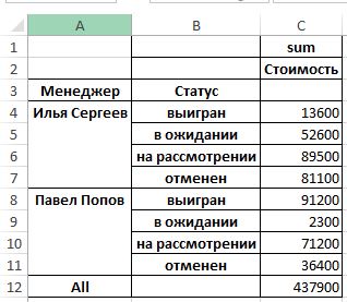
Как мы помним исходной таблице у нас есть столбец "Статус", которому мы присвоили тип категория. Давайте проанализируем работу наших менеджеров этому параметру. Обратите внимание на то, что статусы выводятся именно в том порядке, что мы определили выше:
data_pt = pd.pivot_table(data_pd,index=['Менеджер', 'Статус'], values=['Стоимость'], aggfunc=[np.sum],fill_value=0,margins=True)
Еще одной очень удобной функцией в сводных таблицах Pandas является то, что для каждого типа значений можно выбирать, какую функцию к ним применить. К примеру для "Количество" мы хотим отражать количество продаж, а для "Стоимость" - сумму продаж:
data_pt = pd.pivot_table(data_pd,index=['Менеджер', 'Статус'], values=['Количество', 'Стоимость'], columns=['Продукт'], aggfunc=,fill_value=0)

Также для отдельного значения мы можем использовать несколько агригирующих функций:
data_pt = pd.pivot_table(data_pd,index=['Менеджер', 'Статус'], values=['Количество', 'Стоимость'], columns=['Продукт'], aggfunc=,fill_value=0)

Также мы можем фильтровать данные, выводя только те записи, которые нам интересны. К примеру выведем продажи только менеджера "Илья Сергеев":
data_pt = data_pt.query('Менеджер == ["Илья Сергеев"]')

Или к примеру мы можем вывести только те продажи, у которых статус "выигран" или "в ожидании":
data_pt = data_pt.query('Статус == ["выигран", "в ожидании"]')

На сегодня все. Надеюсь эта статья была вам полезна, спасибо за то что прочитали. Остались вопросы - задавайте в комментариях под статьей.
В этой статье описывается создание и использование двух входных таблиц в Microsoft Excel. Эти таблицы позволяют проверить, как изменения в двух переменных влияют на одну формулу.
Дополнительная информация
При создании таблицы с двумя входными данными в диалоговом окне "Таблица" указываются входные ячейки в полях "Ячейка ввода строк" и "Ячейка ввода столбца".
В Microsoft Office Excel 2007 диалоговое окно "Таблица" называется диалогом таблицы данных.
Чтобы создать простую таблицу с двумя входными данными, выполните следующие действия.
Создайте новую книгу.
В ячейках B15:B19 введите следующие данные:
В ячейках C14:G14 введите следующие данные:
В ячейке B14 введите следующую формулу:
=A14*2+A15
A14 — это входная ячейка столбца (которая заменяет значения 1, 2, 3, 4 и 5), а A15 — ячейку ввода строки (которая заменяет значения 6, 7, 8, 9 и 10). Эти входные ячейки должны находиться за пределами таблицы. они могут содержать или не содержать данные. Так как эта таблица настроена в ячейках B14:G19 и так как A14 и A15 находятся за пределами таблицы, они являются допустимыми входными и входными ячейками строк.
В меню "Данные" щелкните "Таблица".
В Excel 2007 перейдите на вкладку "Данные", выберите "Что если" и "Таблица данных".
В поле "Ячейка ввода строки" введите A15. В поле "Ячейка ввода столбца" введите A14.
Вы увидите следующие результаты:
В качестве примера используйте ячейку C15. Фактические значения, используемые в формуле, — это ячейки B15:B19 (входные ячейки строки) и ячейки C15:G14 (ячейки ввода столбца). Формула со значениями будет иметь значение 1*2+6 (всего 8). Excel внутренне подставляет значения в ячейках ввода строк и столбцов в формулу в ячейке B14.
0 отображается в ячейке B14, хотя ячейка B14 не является числом формата. Чтобы дублировать пустое значение в ячейке B14, выполните следующие действия.
Ссылки
Дополнительные сведения об использовании таблиц данных см. в следующих статьях:
A data table is a range of cells in which you can change values in some of the cells and come up with different answers to a problem. A good example of a data table employs the PMT function with different loan amounts and interest rates to calculate the affordable amount on a home mortgage loan. Experimenting with different values to observe the corresponding variation in results is a common task in data analysis.
In Microsoft Excel, data tables are part of a suite of commands known as What-If analysis tools. When you construct and analyze data tables, you are doing what-if analysis.
What-if analysis is the process of changing the values in cells to see how those changes will affect the outcome of formulas on the worksheet. For example, you can use a data table to vary the interest rate and term length for a loan—to evaluate potential monthly payment amounts.
Note: You can perform faster calculations with data tables and Visual Basic for Applications (VBA). For more information, see Excel What-If Data Tables: Faster calculation with VBA.
Types of what-if analysis
There are three types of what-if analysis tools in Excel: scenarios, data tables, and goal-seek. Scenarios and data tables use sets of input values to calculates possible results. Goal-seek is distinctly different, it uses a single result and calculates possible input values that would produce that result.
Like scenarios, data tables help you explore a set of possible outcomes. Unlike scenarios, data tables show you all the outcomes in one table on one worksheet. Using data tables makes it easy to examine a range of possibilities at a glance. Because you focus on only one or two variables, results are easy to read and share in tabular form.
A data table cannot accommodate more than two variables. If you want to analyze more than two variables, you should instead use scenarios. Although it is limited to only one or two variables (one for the row input cell and one for the column input cell), a data table can include as many different variable values as you want. A scenario can have a maximum of 32 different values, but you can create as many scenarios as you want.
Create either one-variable or two-variable data tables, depending on the number of variables and formulas that you need to test.
One-variable data tables
Use a one-variable data table if you want to see how different values of one variable in one or more formulas will change the results of those formulas. For example, you can use a one-variable data table to see how different interest rates affect a monthly mortgage payment by using the PMT function. You enter the variable values in one column or row, and the outcomes are displayed in an adjacent column or row.
In the following illustration, cell D2 contains the payment formula, =PMT(B3/12,B4,-B5), which refers to the input cell B3.
Two-variable data tables
Use a two-variable data table to see how different values of two variables in one formula will change the results of that formula. For example, you can use a two-variable data table to see how different combinations of interest rates and loan terms will affect a monthly mortgage payment.
In the following illustration, cell C2 contains the payment formula, =PMT(B3/12,B4,-B5), which uses two input cells, B3 and B4.
Data table calculations
Whenever a worksheet recalculates, any data tables will also recalculate—even if there has been no change to the data. To speed up calculation of a worksheet that contains a data table, you can change the Calculation options to automatically recalculate the worksheet but not the data tables. To learn more, see the section Speed up calculation in a worksheet that contains data tables.
A one-variable data table contain its input values either in a single column (column-oriented), or across a row (row-oriented). Any formula in a one-variable data table must refer to only one input cell.
Follow these steps:
Type the list of values that you want to substitute in the input cell—either down one column or across one row. Leave a few empty rows and columns on either side of the values.
Do one of the following:
If the data table is column-oriented (your variable values are in a column), type the formula in the cell one row above and one cell to the right of the column of values. This one-variable data table is column-oriented, and the formula is contained in cell D2.
If you want to examine the effects of various values on other formulas, enter the additional formulas in cells to the right of the first formula.
If the data table is row-oriented (your variable values are in a row), type the formula in the cell one column to the left of the first value and one cell below the row of values.
If you want to examine the effects of various values on other formulas, enter the additional formulas in cells below the first formula.
Select the range of cells that contains the formulas and values that you want to substitute. In the figure above, this range is C2:D5.
On the Data tab, click What-If Analysis > Data Table (in the Data Tools group or Forecast group of Excel 2016).
Do one of the following:
If the data table is column-oriented, enter the cell reference for the input cell in the Column input cell field. In the figure above, the input cell is B3.
If the data table is row-oriented, enter the cell reference for the input cell in the Row input cell field.
Note: After you create your data table, you might want to change the format of the result cells. In the figure, the result cells are formatted as currency.
Formulas that are used in a one-variable data table must refer to the same input cell.
Follow these steps
Do either of these:
If the data table is column-oriented, enter the new formula in a blank cell to the right of an existing formula in the top row of the data table.
If the data table is row-oriented, enter the new formula in a empty cell below an existing formula in the first column of the data table.
Select the range of cells that contains the data table and the new formula.
On the Data tab, click What-If Analysis > Data Table (in the Data Tools group or Forecast group of Excel 2016).
Do either of the following:
If the data table is column-oriented, enter the cell reference for the input cell in the Column input cell box.
If the data table is row-oriented, enter the cell reference for the input cell in the Row input cell box.
A two-variable data table uses a formula that contains two lists of input values. The formula must refer to two different input cells.
Follow these steps:
In a cell on the worksheet, enter the formula that refers to the two input cells.
In the following example—in which the formula starting values are entered in cells B3, B4, and B5, you type the formula =PMT(B3/12,B4,-B5) in cell C2.
Type one list of input values in the same column, below the formula.
In this case, type the different interest rates in cells C3, C4, and C5.
Enter the second list in the same row as the formula—to its right.
Type the loan terms (in months) in cells D2 and E2.
Select the range of cells that contains the formula (C2), both the row and column of values (C3:C5 and D2:E2), and the cells in which you want the calculated values (D3:E5).
In this case, select the range C2:E5.
On the Data tab, in the Data Tools group or Forecast group (in Excel 2016), click What-If Analysis > Data Table (in the Data Tools group or Forecast group of Excel 2016).
In the Row input cell field, enter the reference to the input cell for the input values in the row.
Type cell B4 in the Row input cell box.
In the Column input cell field, enter the reference to the input cell for the input values in the column.
Type B3 in the Column input cell box.
Example of a two-variable data table
A two-variable data table can show how different combinations of interest rates and loan terms will affect a monthly mortgage payment. In the figure here, cell C2 contains the payment formula, =PMT(B3/12,B4,-B5), which uses two input cells, B3 and B4.
When you set this calculation option, no data-table calculations occur when a recalculation is done on the entire workbook. To manually recalculate your data table, select its formulas and then press F9.
Follow these steps to improve calculation performance:
Click File > Options > Formulas.
In the Calculation options section, under Calculate, click Automatic except for data tables.
Tip: Optionally, on the Formulas tab, click the arrow on Calculation Options, then click Automatic Except Data Tables (in the Calculation group).
You can use a few other Excel tools to perform what-if analysis if you have specific goals or larger sets of variable data.
If you know the result to expect from a formula, but don't know precisely what input value the formula needs to get that result, use the Goal-Seek feature. See the article Use Goal Seek to find the result you want by adjusting an input value.
Excel Solver
You can use the Excel Solver add-in to find the optimal value for a set of input variables. Solver works with a group of cells (called decision variables, or simply variable cells) that are used in computing the formulas in the objective and constraint cells. Solver adjusts the values in the decision variable cells to satisfy the limits on constraint cells and produce the result you want for the objective cell. Learn more in this article: Define and solve a problem by using Solver.
By plugging different numbers into a cell, you can quickly come up with different answers to a problem. A great example is using the PMT function with different interest rates and loan periods (in months) to figure out how much of a loan you can afford for a home or a car. You enter your numbers into a range of cells called a data table.
Here, the data table is the range of cells B2:D8. You can change the value in B4, the loan amount, and the monthly payments in column D automatically update. Using a 3.75% interest rate, D2 returns a monthly payment of $1,042.01 using this formula: =PMT(C2/12,$B$3,$B$4).

You can use one or two variables, depending on the number of variables and formulas you want to test.
Use a one-variable test to see how different values of one variable in a formula will change the results. For example, you can change the interest rate for a monthly mortgage payment by using the PMT function. You enter the variable values (the interest rates) in one column or row, and the outcomes are displayed in a nearby column or row.
In this live workbook, cell D2 contains the payment formula =PMT(C2/12,$B$3,$B$4). Cell B3 is the variable cell, where you can plug in a different term length (number of monthly payment periods). In cell D2, the PMT function plugs in the interest rate 3.75%/12, 360 months, and a $225,000 loan, and calculates a $1,042.01 monthly payment.
Use a two-variable test to see how different values of two variables in a formula will change the results. For example, you can test different combinations of interest rates and number of monthly payment periods to calculate a mortgage payment.
In this live workbook, cell C3 contains the payment formula, =PMT($B$3/12,$B$2,B4), which uses two variable cells, B2 and B3. In cell C2, the PMT function plugs in the interest rate 3.875%/12, 360 months, and a $225,000 loan, and calculates a $1,058.03 monthly payment.
Need more help?
You can always ask an expert in the Excel Tech Community or get support in the Answers community.
Читайте также: