
Clustered column excel как построить
Возникало ли у Вас когда-либо желание построить на одной диаграмме графики по двум различным (хотя и связанным) наборам данных? Возможно, Вы хотели видеть количество лидов, одновременно пришедших из нескольких каналов, и уровень конверсии этих каналов. Поместить эти два набора данных на одну диаграмму было бы очень полезно для выяснения закономерностей и определения трендов, наполняющих воронку.
Лид (lead, целевой лид) — потенциальный клиент, тем или иным образом отреагировавший на маркетинговую коммуникацию. Термином лид стало принято обозначать потенциального покупателя, контакт с ним, полученный для последующей менеджерской работы с клиентом.
Но есть проблема. Эти два набора данных имеют совершенно разные размерности оси Y (количество лидов и уровень конверсии) – в итоге график получается очень сомнительный.
К счастью, есть простое решение. Вам потребуется то, что называют вспомогательной осью: с её помощью можно использовать одну общую ось Х и две оси Y различной размерности. Чтобы помочь Вам с решением этой досадной задачи, мы покажем, как добавить вспомогательную ось к диаграмме в Excel на Mac и PC, а также в таблицах Google Doc.
Как добавить вспомогательную ось к диаграмме Excel на Mac
Шаг 1: Вводим данные в таблицу
Пусть в строке 1 будут находиться подписи оси Х, а в строках 2 и 3 – подписи для двух осей Y.

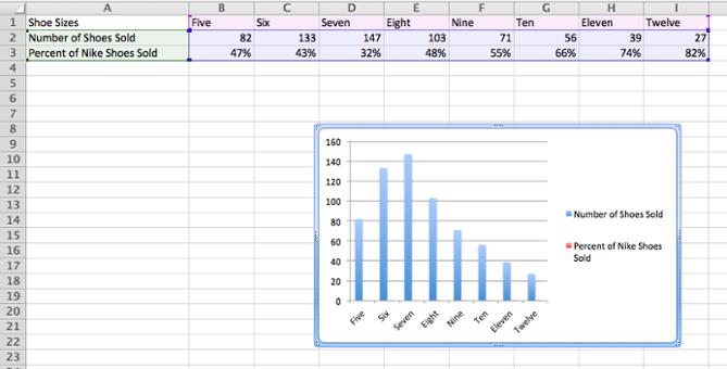
В данном примере: в первой строке указаны размеры обуви, во второй строке – количество проданной обуви, а в третьей – процент проданной обуви.
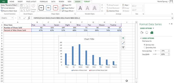
Шаг 2: Создаём диаграмму из имеющихся данных
Выделяем данные, которые нужно показать на диаграмме. Затем в меню нажимаем Диаграммы (Charts), выбираем Гистограмма (Column) и кликаем вариант Гистограмма с группировкой (Clustered Column) вверху слева.
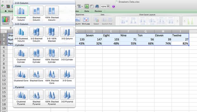
Диаграмма появится чуть ниже набора данных.
Шаг 3: Добавляем вспомогательную ось
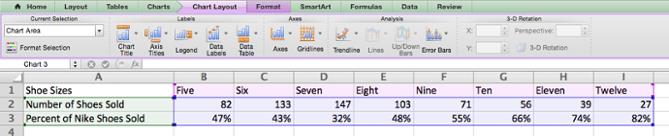
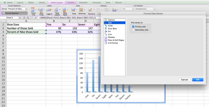
Теперь построим график по вспомогательной оси для данных из строки Percent of Nike Shoes Sold. Выделяем диаграмму, рядом с меню Диаграммы (Charts) должен появиться сиреневый ярлык – Макет диаграммы (Chart Layout). Жмем на него.
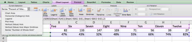
В левом верхнем углу в разделе Текущий фрагмент (Current selection) открываем выпадающий список и выбираем Percent of Nike Shoes Sold или любой другой ряд данных, который нужно отложить по вспомогательной оси.
Когда выбран нужный ряд данных, нажимаем кнопку Формат выделенного (Format Selection) сразу под выпадающим списком. Появится диалоговое окно, в котором можно выбрать вспомогательную ось для построения графика. Если раздел Оси (Axis) не открылся автоматически, кликните по нему в меню слева и выберите вариант Вспомогательная ось (Secondary Axis). После этого нажмите ОК.
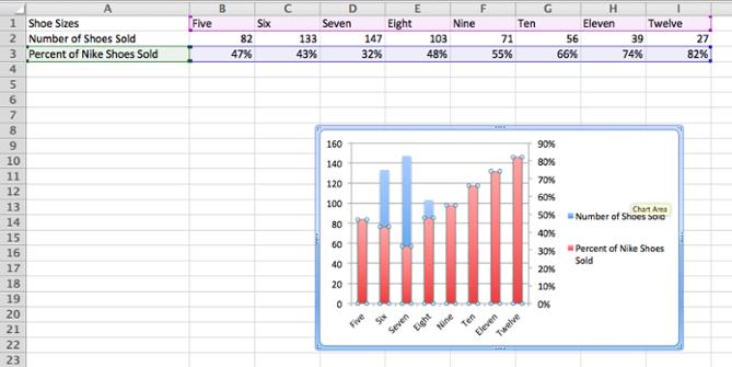
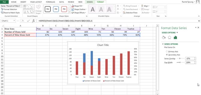
Шаг 4: Настраиваем форматирование
Теперь график Percent of Nike Shoes Sold перекрывает график Number of Shoes Sold. Давайте исправим это.
Выделяем график и снова кликаем зелёную вкладку Диаграммы (Charts). Слева вверху нажимаем График > График (Line > Line).
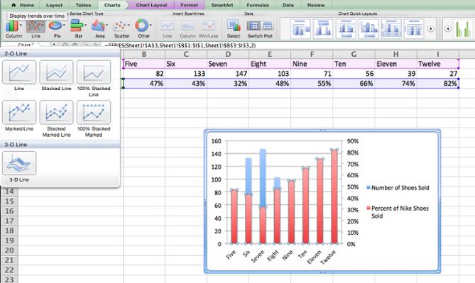
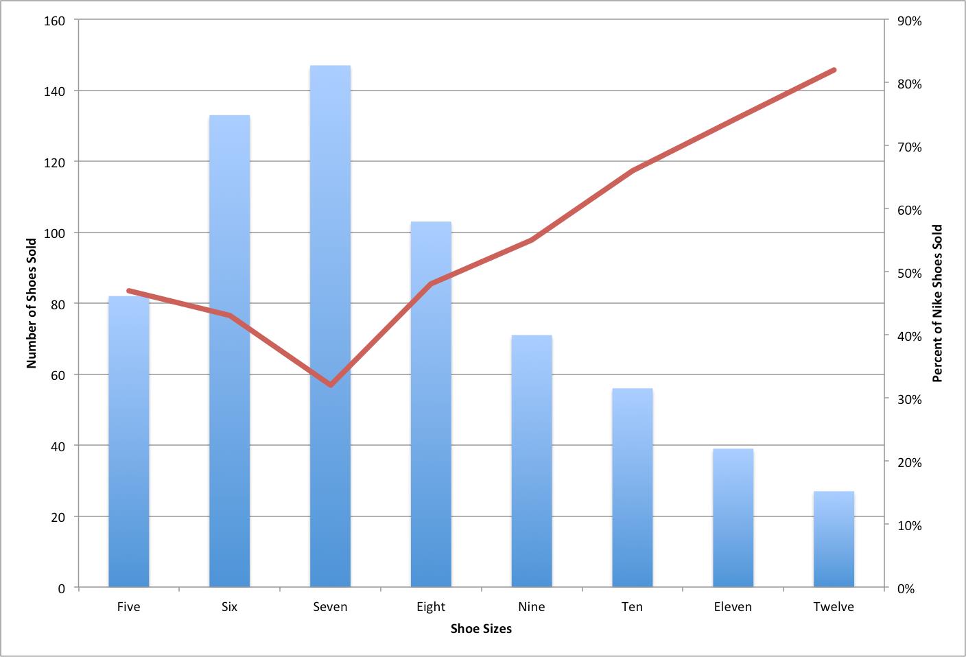
Вуаля! У нас получилась диаграмма, на которой отлично видно количество проданных пар обуви и процент в соответствии с их размерами.
Как добавить вспомогательную ось к диаграмме Excel в Windows
Шаг 1: Добавляем данные на лист
Пусть в строке 1 будут находиться подписи оси Х, а в строках 2 и 3 – подписи для двух осей Y.

Шаг 2: Создаём диаграмму из имеющихся данных
Выделяем данные, которые нужно показать на диаграмме. Затем открываем вкладку Вставка (Insert) и находим раздел Диаграммы (Charts). Кликаем по маленькой иконке с изображением вертикальных линий. Откроется диалоговое окно с несколькими вариантами построения графика на выбор. Выбираем самый первый: Гистограмма с группировкой (Clustered Column).

После щелчка по этой иконке чуть ниже наших данных сразу же появляется диаграмма.

Шаг 3: Добавляем вспомогательную ось
Теперь отобразим данные Percent of Nike Shoes Sold по вспомогательной оси. После того, как была создана диаграмма, на Ленте появилось две дополнительные вкладки: Конструктор (Design) и Формат (Format). Открываем вкладку Формат (Format). В левой части вкладки в разделе Текущий фрагмент (Current Selection) раскрываем выпадающий список Область построения (Chart Area). Выбираем ряд с именем Percent of Nike Shoes Sold – или любой другой ряд, который должен быть построен по вспомогательной оси. Затем нажимаем кнопку Формат выделенного (Format Selection), которая находится сразу под раскрывающимся списком.

В правой части окна появится панель Формат с открытым разделом Параметры ряда (Series Options). Отметьте флажком опцию По вспомогательной оси (Secondary Axis).
Шаг 4: Настраиваем форматирование
Обратите внимание, что график ряда данных Percent of Nike Shoes Sold теперь перекрывает ряд Number of Shoes Sold. Давайте исправим это.
Откройте вкладку Конструктор (Design) и нажмите Изменить тип диаграммы (Change Chart Type).

Появится диалоговое окно. В нижней части окна рядом с Percent of Nike Shoes Sold кликните раскрывающийся список и выберите вариант построения График (Line).

Убедитесь, что рядом с этим выпадающим списком галочкой отмечен параметр Вспомогательная ось (Secondary Axis).

Вуаля! Диаграмма построена!

Как добавить вспомогательную ось в таблицах Google Doc
Шаг 1: Добавляем данные на лист
Пусть в строке 1 будут находиться подписи оси Х, а в строках 2 и 3 – подписи для двух осей Y.
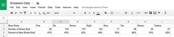
Шаг 2: Создаём диаграмму из имеющихся данных
Выделите данные. Затем зайдите в раздел меню Вставка (Insert) и в открывшемся списке нажмите Диаграмма (Chart) – этот пункт находится ближе к концу списка. Появится вот такое диалоговое окно:
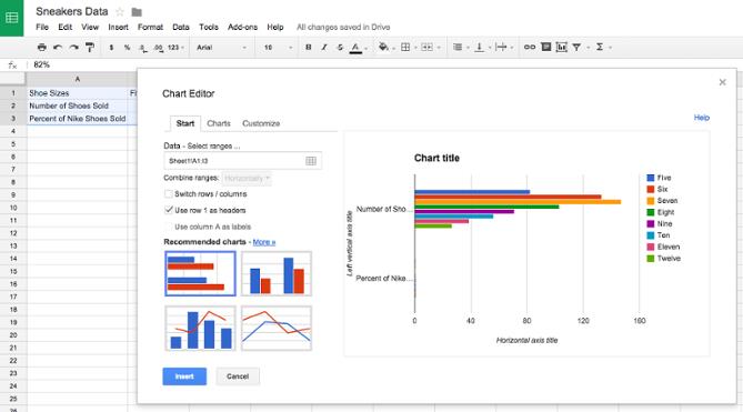
Шаг 3: Добавляем вспомогательную ось
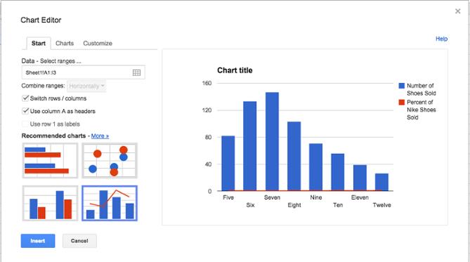
На вкладке Рекомендуем (Start) выберите комбинированную диаграмму, показывающую гистограмму с наложенным на неё линейным графиком. Если этого варианта нет на начальном экране, то нажав ссылку Дополнительно (More) рядом с заголовком Рекомендуем (Recommended charts) выбираем его из полного списка вариантов.
Параметр Заголовки – значения столбца А (Use column A as headers) должен быть отмечен галочкой. Если диаграмма выглядит неправильно, попробуйте изменить параметр Строки / столбцы (Switch rows / columns).
Шаг 4: Настраиваем форматирование
Настало время привести в порядок форматирование. На вкладке Настройка (Customize) пролистываем вниз до раздела Серии (Series). Раскрываем выпадающий список и выбираем имя вспомогательной оси, в нашем случае это Percent of Nike Shoes Sold. В выпадающем списке Ось (Axis) измените Левая ось (Left) на Правая ось (Right). Теперь вспомогательная ось будет отчётливо видна на диаграмме. Далее нажимаем кнопку Вставить (Insert), чтобы разместить диаграмму на листе.
Если вы часто используете Excel, то наверняка знаете о преимуществах графиков не понаслышке. Графическое представление данных оказывается очень полезным, когда нужно наглядно провести сравнение данных или обозначить вектор развития.
Microsoft Excel предлагает множество встроенных типов диаграмм, в том числе гистограммы, линейчатые диаграммы, круговые и другие типы диаграмм. В этой статье мы подробно рассмотрим все детали создания простейших графиков, и кроме того, ближе познакомимся с особым типом диаграммы – каскадная диаграмма в Excel (аналог: диаграмма водопад). Вы узнаете, что представляет собой каскадная диаграмма и насколько полезной она может быть. Вы познаете секрет создания каскадной диаграммы в Excel 2010-2013, а также изучите различные инструменты, которые помогут сделать такую диаграмму буквально за минуту.
И так, давайте начнем совершенствовать свои навыки работы в Excel.
Примечание переводчика: Каскадная диаграмма имеет множество названий. Самые популярные из них: Водопад, Мост, Ступеньки и Летающие кирпичи, также распространены английские варианты – Waterfall и Bridge.
Что такое диаграмма «Водопад»?
Для начала, давайте посмотрим, как же выглядит самая простая диаграмма «Водопад» и чем она может быть полезна.
Диаграмма «Водопад» – это особый тип диаграммы в Excel. Обычно используется для того, чтобы показать, как исходные данные увеличиваются или уменьшаются в результате ряда изменений.
Первый и последний столбцы в обычной каскадной диаграмме показывают суммарные значения. Промежуточные колонки являются плавающими и обычно показывают положительные или отрицательные изменения, происходящие от одного периода к другому, а в конечном итоге общий результат, т.е. суммарное значение. Как правило, колонки окрашены в разные цвета, чтобы наглядно выделить положительные и отрицательные значения. Далее в этой статье мы расскажем о том, как сделать промежуточные столбцы «плавающими».
Диаграмма «Водопад» также называется «Мост«, поскольку плавающие столбцы создают подобие моста, соединяющего крайние значения.
Эти диаграммы очень удобны для аналитических целей. Если вы хотите оценить прибыль компании или доходы от производства продукции, сделать анализ продаж или просто увидеть, как изменилось количество ваших друзей в Facebook за год, каскадная диаграмма в Excel — это то, что вам необходимо.
Как построить каскадную диаграмму (Мост, Водопад) в Excel?
Не тратьте время на поиск каскадной диаграммы в Excel – её там нет. Проблема в том, что в Excel просто нет готового шаблона такой диаграммы. Однако, не сложно создать собственную диаграмму, упорядочив свои данные и используя встроенную в Excel гистограмму с накоплением.
Примечание переводчика: В Excel 2016 Microsoft наконец-то добавила новые типы диаграмм, и среди них Вы найдете диаграмму «Водопад».
Для лучшего понимания, давайте создадим простую таблицу с положительными и отрицательными значениями. В качестве примера возьмем объем продаж. Из таблицы, представленной ниже, видно, что на протяжении нескольких месяцев продажи то росли, то падали относительно начального уровня.

Диаграмма «Мост» в Excel отлично покажет колебания продаж за взятые двенадцать месяцев. Если сейчас применить гистограмму с накоплением к конкретно этим значениям, то ничего похожего на каскадную диаграмму не получится. Поэтому, первое, что нужно сделать, это внимательно переупорядочить имеющиеся данные.
Шаг 1. Изменяем порядок данных в таблице
Первым делом, добавим три дополнительных столбца к исходной таблице в Excel. Назовём их Base, Fall и Rise. Столбец Base будет содержать вычисленное исходное значение для отрезков спада (Fall) и роста (Rise) на диаграмме. Все отрицательные колебания объёма продаж из столбца Sales Flow будут помещены в столбец Fall, а положительные – в столбец Rise.

Также я добавил строку под названием End ниже списка месяцев, чтобы рассчитать итоговый объем продаж за год. На следующем шаге мы заполним эти столбцы нужными значениями.
Шаг 2. Вставляем формулы
Лучший способ заполнить таблицу – вставить нужные формулы в первые ячейки соответствующих столбцов, а затем скопировать их вниз в смежные ячейки, используя маркер автозаполнения.
-
Выбираем ячейку C4 в столбце Fall и вставляем туда следующую формулу:
Замечание: Если Вы хотите, чтобы все значения в каскадной диаграмме лежали выше нуля, то необходимо ввести знак минус (-) перед второй ссылкой на ячейку Е4 в формуле. Минус на минус даст плюс.

Шаг 3. Создаём стандартную гистограмму с накоплением
Теперь все нужные данные рассчитаны, и мы готовы приступить к построению диаграммы:

- Выделите данные, включая заголовки строк и столбцов, кроме столбца Sales Flow.
- Перейдите на вкладку Вставка (Insert), найдите раздел Диаграммы (Charts).
- Кликните Вставить гистограмму (Insert Column Chart) и в выпадающем меню выберите Гистограмма с накоплением (Stacked Column).
Появится диаграмма, пока ещё мало похожая на каскадную. Наша следующая задача – превратить гистограмму с накоплением в диаграмму «Водопад» в Excel.

Шаг 4. Преобразуем гистограмму с накоплением в диаграмму «Водопад»
Пришло время раскрыть секрет. Для того, чтобы преобразовать гистограмму с накоплением в диаграмму «Водопад», Вам просто нужно сделать значения ряда данных Base невидимыми на графике.
После того, как голубые столбцы стали невидимыми, остаётся только удалить Base из легенды, чтобы на диаграмме от этого ряда данных не осталось и следа.

Шаг 5. Настраиваем каскадную диаграмму в Excel
В завершение немного займёмся форматированием. Для начала я сделаю плавающие блоки ярче и выделю начальное (Start) и конечное (End) значения на диаграмме.

- Выделяем ряд данных Fall на диаграмме и открываем вкладку Формат (Format) в группе вкладок Работа с диаграммами (Chart Tools).
- В разделе Стили фигур (Shape Styles) нажимаем Заливка фигуры (Shape Fill).
- В выпадающем меню выбираем нужный цвет.Здесь же можете поэкспериментировать с контуром столбцов или добавить какие-либо особенные эффекты. Для этого используйте меню параметров Контур фигуры (Shape Outline) и Эффекты фигуры (Shape Effects) на вкладке Формат (Format).Далее проделаем то же самое с рядом данных Rise. Что касается столбцов Start и End, то для них нужно выбрать особый цвет, причём эти два столбца должны быть окрашены одинаково.В результате диаграмма будет выглядеть примерно так:
Замечание: Другой способ изменить заливку и контур столбцов на диаграмме – открыть панель Формат ряда данных (Format Data Series) или кликнуть по столбцу правой кнопкой мыши и в появившемся меню выбрать параметры Заливка (Fill) или Контур (Outline).
- Затем можно удалить лишнее расстояние между столбцами, чтобы сблизить их.
- Дважды кликните по одному из столбцов диаграммы, чтобы появилась панель Формат ряда данных (Format Data Series)
- Установите для параметра Боковой зазор (Gap Width) небольшое значение, например, 15%. Закройте панель.Теперь на диаграмме «Водопад» нет ненужных пробелов.
Замечание: Если разница между размерами столбцов очевидна, а точные значения точек данных не так важны, то подписи можно убрать, но тогда следует показать ось Y, чтобы сделать диаграмму понятнее.
Когда закончите с подписями столбцов, можно избавиться от лишних элементов, таких как нулевые значения и легенда диаграммы. Кроме того, можно придумать для диаграммы более содержательное название. О том, как в Excel добавить название к диаграмме, подробно рассказано в одной из предыдущих статей.
Каскадная диаграмма готова! Она значительно отличается от обычных типов диаграмм и предельно понятна, не так ли?

Теперь Вы можете создать целую коллекцию каскадных диаграмм в Excel. Надеюсь, для вас это будет совсем не сложно. Спасибо за внимание!

Clustered Column Charts are the simplest form of vertical column charts in excel available under the Insert menu tab’s Column Chart section. Clustered columns show the growth of all the selected attributes covers the time period allowed by the chart itself. To create this, we simply have to select the data which have been available over a different time period, and we will have columns for each parameter. This is quite useful when we want to show growth.
Excel functions, formula, charts, formatting creating excel dashboard & others
Steps to Make Clustered Column Chart in Excel
To do that, we need to select the entire source Range, including the Headings.
After that, Go to:
Insert tab on the ribbon > Section Charts > > click on More Column Chart> Insert a Clustered Column Chart
Also, we can use the short key; first of all, we need to select all data and then press the short key (Alt+F1) to create a chart in the same sheet or Press the only F11 to create the chart in a separate new sheet.

When we click on more column chart, then we got a new window as below mention. We can choose the format then click on Ok.

How to Make Clustered Column Chart in Excel?
Clustered Column Chart in Excel is very simple and easy to use. Let us understand the working of Clustered Column Chart with some examples.
Excel Advanced Training (16 Courses, 23+ Projects) 16 Online Courses | 23 Hands-on Projects | 140+ Hours | Verifiable Certificate of Completion | Lifetime Access
4.8 (10,560 ratings)
You can download this Clustered Column Chart Excel Template here – Clustered Column Chart Excel Template
There is a summarization of data; this summarization is a company’s performance report, suppose some sales team in different location zone, and they have a target for sale the product. All filed like target, order count, Target, Order Value, Achieved %, Payment received, Discount % is given in the summary; now we can see them in a table as below mention. So we want to display the report by using a cluster column chart.

First of all, select the range. Click on Insert Ribbon > Click on Column chart > More column chart.

Choose the clustered column chart > Click on Ok.

Also, we can use a shortcut key ( alt+F11).

This visualization is default by excel; if we want to change anything so excel allows us to change the data and anything as we want.
If we see on the right hand, so there is an option ‘ + ’ sign, so with the help of the ‘ + ‘ sign, we can display the different chart elements which are we need.

When we use the chart and select then two tabs more display. ‘Design ‘and ‘Format ‘as ribbon,

We can format the chart and color themes layout of the chart with the help of the Design ribbon tab.
Both ribbons are very useful for a chart. E.g., if we change the layout quickly, then just click on the Design tab and click on quick layout and change the layout of the chart.

If we want to change the color, we can use a shortcut to change the style and color of the chat; just click on the chart, and there is an option highlighted, as shown below.

Click on the style you want.
Chart also is given facility to filter the column which we do not need, similarly just click on the chart, at the right side, we can see the filter sign, as showing below mention pictures.

Now we can click on a column that we need to show in the chart.

Again we can change the data range also; Right-click on the chart and select the data option; then, we can change the data also.

We can change the axis horizontally or vertically by just click on the switch row/column. We can also add or remove and edit a file.

We can also format the chart area by just right click on the chart and select the format chart area option.

Then we get a new window on the right side, as shown below.

Just click on the chart option, then we can all options of formatting the chart like chart title, Axis, legend, plot area, series and vertically.

Then click on the option which we want to format.
In the Next Tab, we also format the text.

Some more important things are like add data labels, show trend line in chat; we need to know.
If we want to show data labels as a percentage, just right-click on a column and click on add data labels.

Data Label is added to the chart.

Also, we can show data labels with descriptions. With the help of data callouts. Right-click on column data column labels, click on add data labels and click on add data callouts. The picture is showing below mentioned.

Data Callouts are added to the chart.

Sometimes we need trend analysis also on a chart. So right-click on data labels and add the trend line.

A Trendline is added to the chart.

We can also format the trend line.

If we want to format the gridlines, then right-click on Gridlines and click on format gridlines.


Right Click on Gridlines and click on Add Miner Gridlines.

A miner Gridlines is added to it.

Right Click on Gridlines and click on Format Axis.


Finally, the Clustered Column Chart looks as given below.

Pros and Cons of a Clustered Column Chart in Excel
Following are the Pros and Cons:
- Since a Clustered Column chart is a default Excel chart type, at least until you set another chart type as a default type
- It can be understood by any person and will look presentable who is not much more familiar with the chart.
- It helps us to make a summarization of a huge data in the visualization, so easily we can understand the report.
- It’s visually complex when we add more categories or series.
- At one time more difficult to compare a single series across categories.
Things to be Remember
- All columns and labels should be filled with various colors to highlight the data in our chart easily.
- Use self-explanatory chart titles, axes titles. So by the title name, one can understand the report.
- If the data is relevant for this chart, then use this chart; otherwise, the data is related to different categories; we can choose another chart type that is representable.
- No need of using extra formatting so that anyone can see and analyze all points clearly.
Recommended Articles
This has been a guide to a Clustered Column Chart in Excel. Here we discuss how to create the Clustered Column Chart in Excel with excel examples and downloadable excel templates. You may also look at these useful functions in Excel –

Clustered Bar Chart in excel is shown as horizontal bars laid parallel to X-Axis, which is also used for comparing the values across different categories. We can access the Clustered Bar Chart from the Insert menu under the Charts section in the Bar Chart Section available in both 2D and 3D types of charts. To create Clustered Bar, we must have 2 values for a one-parameter where we can compare those values before and after or in a different time frame.
Excel functions, formula, charts, formatting creating excel dashboard & others
The below image shows the difference between the COLUMN & BAR charts.

The main difference is showing the values horizontally and vertically at an interchanged axis.
Types of Bar Chart in Excel
There are a total of 5 types of bar charts available in excel 2010.
- 2-D Bar and 2-D stacked Bar chart
- 3-D Bar and 3-d stacked Bar chart
- Cylinder Bar chart
- Cone Bar chart
- Pyramid Bar chart
How to Create a Clustered Bar Chart in Excel?
It is very simple and easy to use. Let us now see how to create a Clustered Bar Chart with the help of some examples.
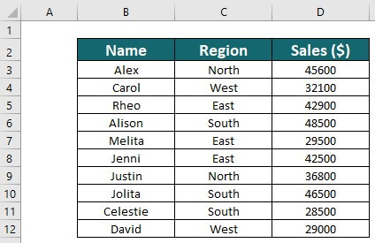
In this example, I have 4 years of data with a break-up each quarter each year.
Excel Advanced Training (16 Courses, 23+ Projects) 16 Online Courses | 23 Hands-on Projects | 140+ Hours | Verifiable Certificate of Completion | Lifetime Access
4.8 (10,560 ratings)
Step 1: Dataset should look like this.

Step 2: Select Data > Go to Insert > Bar Chart > Clustered Bar Chart.

As soon as you insert the chart, it will look like this.

Oh! This looks ugly, man. We need to beautify it.
Step 3: Right click on the bar and select format data series.

Go to fill and select Vary colors by point.

Step 4: As of now, it looks better than the previous one. We need to format our vertical axis. We need to rearrange the data as shown in the below image.

Step 5: Once the data has rearranged your chart, it looks like this.

Step 6: Right click on the bar and select format data series.

Make the Gap Width 0%. Series Overlap to 0%.

Ok, our clustered bar chart is ready, and we can just read the numbers from the graph itself.
Interpretation of the Chart:
- Q1 of 2015 is the highest sales period where it has generated revenue of more than 12 lakhs.
- Q1 of 2016 is the lowest point in revenue generation. That particular quarter generated only 5.14 lakhs.
- In 2014 after a dismal show in Q2 & Q3, there is a steep rise in revenue. Currently, this quarter’s revenue is the second-highest revenue period.
Our final looks like this.

I am using Target vs Actual data for this example.
Step 1: Arrange the data in the below format.

Step 2: Insert the chart from the insert section. Go to Bar Chart and then select Clustered Bar Chart.

Initially, your chart looks like this.

Do the formatting by following the below steps.
- Right click on the chart and choose Select Data.


- Apply to formate as we have done in the previous one, and after that, your chart looks like this. Change the chart type for the Target series to present better. Select the target bar, go-to design, and click on Change Chart Type.


- So our chart is ready to convey the message now, and it looks like this.

Advantages
- Easy to make and understand.
- We can compare the multiple categories subcategories easily.
- We can spot the changes very easily.
- Very useful if the data categories are small.
Disadvantages
- Creates confusions if the data is too large.
- There are chances of overlapping of many subseries.
- I May not be able to fit everything in one chart.
Things to Remember About Clustered Bar Chart
- Arrange the data before creating a Clustered Bar Chart.
- If the data is too large, chose a different chart.
- Avoid 3D effects.
- Construct the chart carefully so that it will not overlap with other categories.
Recommended Articles
This has been a guide to Clustered Bar Chart. Here we discuss its types and how to create Excel Clustered Bar Chart along with excel examples and a downloadable excel template. You may also look at these useful charts in excel –

A stacked bar chart is a type of bar chart used in excel for the graphical representation of part-to-whole comparison over time. This helps you to represent data in a stacked manner. This type of graph is suitable for data that is represented in different parts and one as a whole. The gradual variation of different variables can be picturized using this.
Excel functions, formula, charts, formatting creating excel dashboard & others
The stacked bar graph can be implemented in 2D or 3D format. From the Insert menu, the chart option will provide different types of charts. The stacked bar chart comes under the bar chart. Two types of stacked bar charts are available. Stacked bar chart and 100% stacked bar chart. The stacked bar chart represents the given data directly, but a 100% stacked bar chart will represent the given data as the percentage of data that contribute to a total volume in a different category.
A variety of bar charts are available, and according to the data you want to represent, the suitable one can be selected. 2D and 3D stacked bar charts are given below. The 100% stacked bar chart is also available in 2D and 3D style.
How to Create a Stacked Bar Chart in Excel?
The stacked Bar Chart in Excel is very simple and easy to create. Let us now see how to create a Stacked Bar Chart in Excel with the help of some examples.
A dietitian gives fruit conception of three different patients. Different fruits and their conception are given. Since the data consist of three different persons and five different fruits, a stacked bar chart will be suitable to represent the data. Let’s see how this can be graphically represented as a stacked bar chart.
- John, Joe, Jane are the 3 different patients, and the fruits conception are given as below.

- Select the column Category and 3 patient’s quantity of conception. Select Insert from the menu.

- Select the See All Charts option and get more charts types. Click on the small down arrow icon.

- You will get a new window to select the type of graph. The recommended charts and All Charts tab will be shown. Click on the All Charts tab.

- You can see a different type of graph is listed below it. Select the Bar graph since we are going to create a stacked bar chart.

- Different bar charts will be listed. Select the Stacked Bar graph from the list.

- Below are the two format styles for the stacked bar chart. Click on any one of the given styles. Here we have selected the first one and then press the OK button.

- The graph will be inserted into the worksheet. And it is given below.

- For more settings, you can press the “+” symbol right next to the chart. You can insert the axis name, heading, change color, etc.


Three different colors represent three persons. The bar next to each fruit shows its conception by different patients. From the graph, it is easy to find who used a particular fruit more, who consumes more fruits, which fruit consumes more apart from the given five.
Sales report of different brands is given. Brand names and sales are done for 3 years 2010, 2011, 2012. Let’s try to create a 3-D stacked bar chart using this.
- Sales done for different brands and years are given as below.
- Select the data and go to the chart option from the Insert menu. Click on the bar chart select a 3-D Stacked Bar chart from the given styles.

- The chart will be inserted for the selected data as below.

- By clicking on the title, you can change the tile.

- Extra settings to change the color and X, Y-axis names, etc.
- The axis name can be set by clicking on the “+” symbol and select Axis Titles.

- The chart for the sales report will finally look as below.

The sales in different years are shown in 3 different colors. The bar corresponding to each brand shows sales done for a particular one.
In this example, we are trying to graphically represent the same data given above in a 3-D stacked bar chart.
Excel Advanced Training (16 Courses, 23+ Projects) 16 Online Courses | 23 Hands-on Projects | 140+ Hours | Verifiable Certificate of Completion | Lifetime Access
4.8 (10,568 ratings)
- The data table looks as below with brand names and sales done for different periods.
- By selecting the cell from B2: E11, go to the Insert menu. Click on the Chart option. From Bar Charts, select the 100% Stacked Bar Chart from 2-D or 3-D style. Here we selected form 2-D style.

- The graph will be inserted into the worksheet. And it is given below.

- The color variations can also be set by right-clicking on the inserted graph. The color fill options will be available. The final output will be as below.

The Y-axis values are given in percentage. And the values are represented in a percentage of 100 as a cumulative.
Things to Remember About Stacked Bar Chart in Excel
- The data given as different parts and cumulated volume can be easily represented using a stacked bar chart.
- Multiple data of gradual variation of data for a single variable can effectively visualize by this type of graphs.
- Stacked bar charts are helpful when you want to compare total and one part as well.
- According to the data set, select the suitable graph type.
Recommended Articles
This has been a guide to Stacked Bar Chart in Excel. Here we discuss how to create a Stacked Bar Chart in excel along with excel examples and a downloadable excel template. You may also look at these suggested articles –
Читайте также: