
Break links excel где
There are many ways to create a hyperlink in Excel. To link to a certain web page, you can simply type its URL in a cell, hit Enter, and Microsoft Excel will automatically convert the entry into a clickable hyperlink. To link to another worksheet or a specific location in another Excel file, you can use the Hyperlink context menu or Ctrl + K shortcut. If you plan to insert many identical or similar links, the fastest way is to use a Hyperlink formula, which makes it easier to create, copy and edit hyperlinks in Excel.
Excel HYPERLINK function - syntax and basic uses
The HYPERLINK function in Excel is used to create a reference (shortcut) that directs the user to the specified location in the same document or opens another document or web-page. By using a Hyperlink formula, you can link to the following items:
- A specific place such as a cell or named range in an Excel file (in the existing sheet or in another worksheet or workbook)
- Word, PowerPoint or other document stored on your hard disk drive, local network or online
- Bookmark in a Word document
- Web-page on the Internet or intranet
- Email address to create a new message
The function is available in all versions of Excel for Office 365, Excel 2019, Excel 2016, Excel 2013, Excel 2010, Excel 2007, Excel 2003, Excel XP, and Excel 2000. In Excel Online, the HYPERLINK function can only be used for web addresses (URLs).
The syntax of the HYPERLINK function is as follows:
-
Link_location (required) is the path to the web-page or file to be opened.
Link_location can be supplied as a reference to a cell containing the link or a text string enclosed in quotation marks that contains a path to a file stored on a local drive, UNC path on a server, or URL on the Internet or intranet.
If the specified link path does not exist or is broken, a Hyperlink formula will throw an error when you click the cell.
Clicking a cell with a Hyperlink formula opens the file or web-page specified in the link_location argument.
Below, you can see the simplest example of an Excel Hyperlink formula, where A2 contains friendly_name and B2 contains link_location:

The result may look something similar to this:
More formula examples demonstrating other uses of the Excel HYPERLINK function follow below.
How to use HYPERLINK in Excel - formula examples
Moving from theory to practice, let's see how you can use the HYPERLINK function to open various documents directly from your worksheets. We will also discuss a more complex formula where Excel HYPERLINK is used in a combination with a few other functions to accomplish a non-trivial challenging task.
How to link to sheets, files, web-pages and other items
The Excel HYPERLINK function enables you to insert clickable hyperlinks of a few different types depending on what value you supply to the link_location argument.
Hyperlink to another worksheet
The above formula creates a hyperlink with the jump text "Sheet2" that opens Sheet2 in the current workbook.
If the worksheet name includes spaces or non-alphabetical characters, it must be enclosed in single quotation marks, like this:
In the same way, you can make a hyperlink to another cell in the same sheet. For example, to insert a hyperlink that will take you to cell A1 in the same worksheet, use a formula similar to this:
Hyperlink to a different workbook
To create a hyperlink to another workbook, you need to specify the full path to the target workbook in the following format:
=HYPERLINK("D:\Source data\Book3.xlsx", "Book3")
To land on a specific sheet and even in a specific cell, use this format:
For example, to add a hyperlink titled "Book3" that opens Sheet2 in Book3 stored in the Source data folder on drive D, use this formula:
=HYPERLINK("[D:\Source data\Book3.xlsx]Sheet2!A1", "Book3")
If you plan to move your workbooks to another location soon, you can create a relative link like this:
=HYPERLINK("Source data\Book3.xlsx", "Book3")
When you move the files, the relative hyperlink will continue working as long as the relative path to the target workbook remains unchanged. For more information, please see Absolute and relative hyperlinks in Excel.
Hyperlink to a named range
If you are making a hyperlink to a worksheet-level name, include the full path to the target name:
For instance, to insert a link to a range named "Source_data" stored on Sheet1 in Book1, use this formula:
=HYPERLINK("[D:\Excel files\Book1.xlsx]Sheet1!Source_data","Source data")
If you are referencing a workbook-level name, the sheet name does not need to be included, for example:
=HYPERLINK("[D:\Excel files\Book1.xlsx]Source_data","Source data")
Hyperlink to open a file stored on a hard disk drive
To create a link that will open another document, specify the full path to that document in this format:
For example, to open the Word document named Price list that is stored in the Word files folder on drive D, you use the following formula:
=HYPERLINK("D:\Word files\Price list.docx","Price list")
Hyperlink to a bookmark in a Word document
To make a hyperlink to a specific location in a Word document, enclose the document path in [square brackets] and use a bookmark to define the location you want to navigate to.
For example, the following formula adds a hyperlink to the bookmark named Subscription_prices in Price list.docx:
=HYPERLINK("[D:\Word files\Price list.docx]Subscription_prices","Price list")
Hyperlink to a file on a network drive
To open a file stored in your local network, supply the path to that file in the Universal Naming Convention format (UNC) that uses double backslashes to precede the name of the server, like this:
The below formula creates a hyperlink titled "Price list" that will open the Price list.xlsx workbook stored on SERVER1 in Svetlana folder:
=HYPERLINK("\\SERVER1\Svetlana\Price list.xlsx", "Price list")
To open an Excel file at a specific worksheet, enclose the path to the file in [square brackets] and include the sheet name followed by the exclamation point (!) and the referenced cell:
=HYPERLINK("[\\SERVER1\Svetlana\Price list.xlsx]Sheet4!A1", "Price list")
Hyperlink to a web page
To create a hyperlink to a web-page on the Internet or intranet, supply its URL enclosed in quotation marks, like this:
=HYPERLINK("https://www.ablebits.com","Go to Ablebits.com")
The above formula inserts a hyperlink, titled "Go to Ablebits.com", that opens the home page of our web-site.
Hyperlink to send an email
To create a new message to a specific recipient, provide an email address in this format:
=HYPERLINK("mailto:support@ablebits.com","Drop us an email")
The above formula adds a hyperlink titled "Drop us an email", and clicking the link creates a new message to our support team.
Vlookup and create a hyperlink to the first match
When working with large datasets, you may often find yourself in a situation when you need to look up a specific value and return the corresponding data from another column. For this, you use either the VLOOKUP function or a more powerful INDEX MATCH combination.
But what if you not only want to pull a matching value but also jump to the position of that value in the source dataset to have a look at other details in the same row? This can be done by using the Excel HYPERLINK function with some help from CELL, INDEX and MATCH.
The generic formula to make a hyperlink to the first match is as follows:
To see the above formula in action, consider the following example. Supposing, you have a list of vendors in column A, and the sold products in column C. You aim to pull the first product sold by a given vendor and make a hyperlink to some cell in that row so you can review all other details associated with that particular order.
With the lookup value in cell E2, vendor list (lookup range) in A2:A10, and product list (return range) in C2:C10, the formula takes the following shape:

As shown in the screenshot below, the formula pulls the matching value and converts it into a clickable hyperlink that directs the user to the position of the first match in the original dataset.
If you are working with long rows of data, it might be more convenient to have the hyperlink point to the first cell in the row where the match is found. For this, you simply set the return range in the first INDEX MATCH combination to column A ($A$2:$A$10 in this example):

This formula will take you to the first occurrence of the lookup value ("Adam") in the dataset:
How this formula works
Those of you who are familiar with the INDEX MATCH formula as a more versatile alternative to Excel VLOOKUP, have probably already figured out the overall logic.
At the core, you use the classic INDEX MATCH combination to locate the first occurrence of the lookup value in the lookup range:
You can find full details on how this formula works by following the above link. Below, we will outline the key points:
- The MATCH function determines the position of "Adam" (lookup value) in range A2:A10 (lookup range), and returns 3.
- The result of MATCH is passed to the row_num argument of the INDEX function instructing it to return the value from the 3 rd row in range C2:C10 (return range). And the INDEX function returns "Lemons".
This way, you get the friendly_name argument of your Hyperlink formula.
Note. Please notice the use of absolute cell references to fix the lookup and return ranges. This is critical if you plan to insert more than one hyperlink by copying the formula.
How to edit multiple hyperlinks at a time
As mentioned in the beginning of this tutorial, one of the most useful benefits of formula-driven hyperlinks is the ability to edit multiple Hyperlink formulas in one go by using Excel's Replace All feature.
- Press Ctrl + H to open the Replace tab of the Find and Replace dialog.
- In the right-hand part of the dialog box, click the Options button.
- In the Find what box, type the text you want to change ("old-website.com" in this example).
- In the Within drop-down list, select either Sheet or Workbook depending on whether you want to change hyperlinks on the current worksheet only or in all sheets of the current workbook.
- In the Look in drop-down list, select Formulas.
- As an extra precaution, click the Find All button first, and Excel will display a list of all formulas containing the search text:
- Look though the search results to make sure you want to change all of the found formulas. If you do, proceed to the next step, otherwise refine the search.
- In the Replace with box, type the new text ("new-website.com" in this example).
- Click the Replace All button. Excel will replace the specified text in all found hyperlinks and notify you how many changes have been made.
- Click the Close button to close the dialog. Done!
In a similar fashion, you can edit the link text (friendly_name) in all Hyperlink formulas at the same time. When doing so, be sure to check that the text to be replaced in friendly_name does not appear anywhere in link_location so that you won't break the formulas.
Excel HYPERLINK not working - reasons and solutions
The most common reason for a Hyperlink formula not working (and the first thing for you to check!) is a non-existent or broken path in the link_location argument. If it's not the case, check out the following two things:
- If the link destination does not open when you click a hyperlink, make sure the link location is supplied in the proper format. Formula examples to create different hyperlink types can be found here.
- If instead of the link text an error such as VALUE! or N/A appears in a cell, most likely the problem is with the friendly_name argument of your Hyperlink formula.
This is how you create hyperlinks using the Excel HYPERLINK function. I thank you for reading and hope to see you on our blog next week!
There are two different methods to break external links in the Excel worksheet. The first method is to copy and paste as a value method, which is very simple. The second method is a little different. First, we need to go to the “DATA” tab and click “Edit Links,” and find the option to break the link.
2 Different Methods to Break External Links in Excel

Now, we must paste them as values.

We can see here that this value does not contain any links. It shows only value.

The second method is a little different. In this method, we must go to the “DATA” tab and click on “Edit Links.”

Now, we can see the below-shown dialogue box.

Here we can see all the available external links. We can update the values, open-source files, and many other things. Apart from all these, we can also break these links.
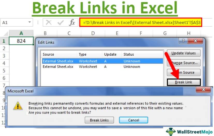
Now, we will click on the “Break Link.”

As soon as we click on “Break Link,” we may see the dialogue box as shown below.

If we wish to break all the links at once, we need to select all the links and click on “Break Links.”
Things to Remember
- It is dangerous to have links to external sources in Excel.
- Once we break the link in Excel, we cannot undo the action.
- Using *.xl can cover all kinds of file extensions.
Recommended Articles
This article has been a guide to Break Links in Excel. Here, we discuss how to break external links in Excel using two methods, 1. Copy Paste as Value, and 2. Edit Links Option Tab, along with practical examples. You may learn more about Excel from the following articles: –
External links are also known as the external references in excel, when we use any formula in excel and refer to any other workbook apart from the workbook with formula then the new workbook being referred to is the external link to the formula, In Simple words when we give a link or apply a formula from another workbook then it is called an external link.
If our formula reads like the below, then it is an external link.

‘C:UsersAdmin_2.Dell-PCDesktop: This is the path to that sheet on the computer.
[External Sheet.xlsx]: This is the Workbook name in that path.
Vlookup Sheet: This is the worksheet name in that workbook.
$C$1:$D$25: This is the range in that sheet.
Types of External Links in Excel
- Links within the same worksheet.
- Links from different worksheets but from the same workbook.
- Links from a different workbook
These types of links are within the same worksheet. In a workbook, there are many sheets. This type of link specifies only the cell name.
For Example: If you are in the cell B2 and if the formula bar reads A1, that means whatever happens in the A1 cell will reflect in the cell B2.

Ok, this is just the simple link within the same sheet.
These types of links are within the same workbook but from different sheets.
For Example, in a workbook, there are two sheets, and right now, I am in sheet1 and giving a link from sheet2.

This type of link is called external links. This means this is altogether from a different workbook itself.
For Example, if I have, I am giving a link from another workbook called “Book1” then, first it will show the workbook name, sheet name, and then the cell name.

How to Find, Edit, and Remove External Links in Excel?
There are multiple ways we can find external links in the excel workbook. As soon as we open a worksheet, we will get the below dialogue box before we get inside the workbook, and that is the indication that this workbook has external links.

Ok, let me explain the methods to find external links in excel.
If there are external, links the link must have included its path or URL to the referring workbook. One this common in all the links is the operator symbol “[“
Below are the steps used to find external links using find & replace method –
-
Select the sheet press Ctrl + F (shortcut to find external links).


Note: If your data includes the symbol, [then it will also convert to values.
A cell with external references includes a workbook name, i.e., workbook name, and the type of workbook is included.
The common file extensions are .xlsx , .xls , .xlsm , .xlb.
Step 1: Select the sheet press Ctrl + F (shortcut to find external links).

Step 2: Now enter .xlsx and click on find all.

This will show all the external link cells.
This is the most direct option we have in excel. It will highlight only the external link, unlike in Method 1 & 2. In this method, we can edit the link in excel, break, or delete and remove external links.
The Edit link option in excel is available under the Data Tab.

Step1: Select the cells you want to edit, break, or delete the link cells.
Step 2: Now click on Edit Links in Excel. There are a couple of options available here.
- Update Values: This will update any changed values from the linked sheet.
- Change Source: This will change the source file.
- Open Source: This will open the source file instantly.
- Break Link: This will permanently delete the formula, remove the external link, and retain only the values. Once this is done, we cannot undo it.
- Check Status: This will check the status of the link.
Note: Sometimes, even if there is an external source still these methods won’t show anything, but we need to manually check graphs, charts, names ranges, data validation, condition formatting Condition Formatting Conditional formatting is a technique in Excel that allows us to format cells in a worksheet based on certain conditions. It can be found in the styles section of the Home tab. read more , chart title, shapes, or objects.
Things to Remember
- We can find external links by using VBA codeVBA CodeVBA code refers to a set of instructions written by the user in the Visual Basic Applications programming language on a Visual Basic Editor (VBE) to perform a specific task.read more . Search on the internet to explore this.
- If the external link is given to shapes, we need to look for it manually.
- External formula links will not show the results in the case of SUMIF Formulas in ExcelSUMIF Formulas In ExcelThe SUMIF Excel function calculates the sum of a range of cells based on given criteria. The criteria can include dates, numbers, and text. For example, the formula “=SUMIF(B1:B5, “ <=12”)” adds the values in the cell range B1:B5, which are less than or equal to 12.read more , SUMIFS & COUNTIF formulasCOUNTIF FormulasThe COUNTIF function in Excel counts the number of cells within a range based on pre-defined criteria. It is used to count cells that include dates, numbers, or text. For example, COUNTIF(A1:A10,”Trump”) will count the number of cells within the range A1:A10 that contain the text “Trump”read more . It will show the values only if the sourced file is opened.
- If excel still shows an external link prompt, we need to check all the formatting, charts, validation, etc. manually.
- Keeping external links will be helpful in case of auto-updating from the other sheet.
Recommended Articles
This has been a guide to External Links in Excel. Here we discuss types of links and dealing with external links, how to find, edit, and remove External links in Excel along with excel example and downloadable excel templates. You may also look at these useful functions in excel –
Keeping track of all external references in a workbook can be challenging. This tutorial will teach you a few useful techniques to find links to external sources in Excel formulas, objects and charts and shows how to break external links.
When you want to pull data from one file to another, the fastest way is to refer to the source workbook. Such external links, or external references, are a very common practice in Excel. After completing a particular task, however, you may want to find and probably break those links. Astonishingly, there is no quick way to locate all links in a workbook at once. Depending on exactly where the references are located - in formulas, defined names, objects, or charts - you will have you use different methods.
How to find cells with external links in Excel
- In your worksheet, press Ctrl + F to open the Find and Replace dialog.
- Click the Options button.
- In the Find what box, type .xl. This way, you will search for all possible Excel file formats including .xls (older workbooks) .xlsx (modern workbooks) .xlsm (macro-enabled workbooks), etc.
- In the Within box, select either Workbook to search in all tabs or Sheet to look in the current worksheet only.
- In the Look in box, choose Formulas.
- Click the Find All button.
That's it! You've got a list of cells that have any external references in them.

And these useful tips will help you manage the results:
- To select acell that contains an external link, click the cell address in the Cell
- To group the found links the way you want, click the corresponding column header, for example, Sheet or Formula.
- To select all cells with external references, place the cursor anywhere within the results and press Ctrl + A . This will select both the results in the Find and Replace dialog box and the cells in the workbook.
Note. With Find and Replace you can only identify external links in cells. If you've removed all external references from formulas but Excel still says there are links to external workbooks, then check other possible locations discussed below.
How to find links in Excel named ranges (defined names)
Excel pros often name ranges and individual cells to make their formulas easier to write, read, and understand. Data validation drop-down lists are also easier to create with named ranges, which in turn may refer to outside data. To take care of such cases, check for external links in Excel names:
- On the Formulas tab, in the Defined Names group, click Name Manager or press the Ctrl + F3 key combination.
- In the list of names, check the Refers Tocolumn for external links. References to other workbooks are enclosed in square brackets like [Source_data.xlsx].

How to identify external links in Excel objects
If you've linked objects such as shapes, text boxes, WordArt and the like to other Excel files, then you can use the Go To Special feature to locate such links:
- On the Hometab, in the Formats group, click Find & Select >Go to Special. Or press F5 to open for the Go To dialog, and then click Special… .
- In the Go To Special dialog box, select Objects and click OK. This will select all objects on the active sheet.

If an object is linked to a specific cell, you can see an external reference in the formula bar:

If an object is linked to a file, then hover over the object with your mouse to see where it points to:

Note. If an object is linked to a whole file rather than an individual cell, such link cannot be broken by using the Edit Links feature. To remove the link, right-click the object and select Remove link from the context menu.
How to find links to other files in Excel charts
In case external links are used in a chart title or data series, you can locate them in this way:
- On the graph, click the chart title or data series you wish to check.
- In the formula bar, look for a reference to another Excel file.
External reference in chart title:

External link in chart data series:

If your chart contains several data series, you can quickly move between them in this way:
- Select the target chart.
- Go to the Format tab >Current Selection group, click the arrow next to the Chart Elements box, and select the data series of interest.

How to find external links in Pivot Tables
Most often a PivotTable is created using the data in the same workbook. But sometimes, the source data resides in an outside file. To find the exact location of your PivotTable's source data, perform these steps:
- Click any cell within the Pivot Table.
- On the PivotTable Analyze tab, in the Data group, click the Change Data Source button.
How to enable links to external workbooks in Excel
When you open a workbook with links to other files for the first time, Excel shows a security warning informing you that the file contains links to external data. To allow the links to update, simply click the Enable Content button.
![]()
On subsequent openings of the same file, you will be presented with the following prompt asking if you want to update the links. If you trust the linked documents and want to pull the latest data, click Update.

Control the security prompt about updating links
By default, Excel asks whether or not to update external references every time you open a workbook. However, you can control whether the message appears and whether the links are updated or not.
- On the Datatab, in the Queries & Connections group, click Edit Links.
- In the lower-left corner of the Edit Links dialog box, click Startup Prompt….
- Let users choose to display the alert or not (default).
- Don't display the alert and don't update automatic links - it makes sense to choose this option when you are sharing a workbook with other people who do not have access to the source files.
- Don't display the alert and update links - you can choose this setting when you completely trust the sources.

Change security setting for external links
You can also set links to other files to be updated automatically in a particular workbook without getting a security warning by changing the Trust Center security settings:
- In the target workbook, click the File tab >Options.
- In the Excel Options dialog box, click Trust Center >Trust Center Settings.

Please note that automatic updating of links to unknown files can be harmful and therefore is not recommended. Enable it only when you are 100% confident in the security of the outside data. Or, turn on this option temporarily, and then return to the default Prompt user on automatic update for Workbook Links setting.

Note. Regardless which option you choose, Excel will still display the below prompt if the workbook contains invalid or broken links.
How to break external links in Excel
In Excel, breaking a link to another workbook means replacing an external reference with its current value.
For example, if you break the following external reference, it will be replaced with the value that is currently in cell A1 on the Jan sheet in the Source data workbook:
If you break an external link in the below formula, the formula will be changed to its calculated value, whatever it is:
Note. Because breaking links is the action that cannot be undone, it may be wise to save a backup copy of your workbook first.
To break external links in Excel, this is what you need to do:
-
On the Data tab, in the Queries &Connections group, click the Edit Links button.

- To select multiple links, click on each one individually while holding down the Ctrl key.
- To select all links, press the Ctrl + A shortcut .

Note. Under ideal circumstances, this feature should remove all external links in a workbook. Unfortunately, we do not live in a perfect world :( Some links to outside data, e.g. external source data in Pivot Tables, are not shown in the Edit Links dialog while others cannot be broken. If the Edit Links button is grayed out in your workbook but you are still getting a prompt about external data, then you will have to check each possible place where external references may be lurking (such as objects, charts, etc.) and change or remove the links manually.
Get a list of all external links in a workbook
To get a list of all external sources that your workbook refers to, you can use one of the following methods.
Traditional approach
This will display the following information:
- Source - the name of the linked file
- Type - the link type: a workbook or worksheet
- Update - whether the link updates automatically or manually
- Status - the status of the link such as OK, Source is Open, Warning, Unknown, etc. To get the most recent info, click the Check Status button on the right.

Very quick and straightforward, this method is not very convenient though. To see the location of the source file, you need to click each link, one at a time.
Dynamic arrays and Excel 4.0 macros.
A very cute trick suggested by Bob Ulmas in his book "This isn't Excel, it's Magic!" can help you retrieve the locations of all source files in one go. The solution combines the recently introduced dynamic arrays with the good old Excel 4.0 macros.
To generate a list of all external references in a given workbook, this is what you need to do:
Step 1. Create a new name that references the macro
To be able to use a built-in Excel 4.0 macro in a formula, you need to create a name referencing the macro. Here's how:
- On the Formulas tab, in the Defined Names group, click Name Manager. Or simply press the Ctrl + F3 shortcut.
- In the Name Manager dialog window, click the New…
- In the New Name dialog window, type some meaningful name, say GetLinks, in the Name box and the following formula in the Refers to box: =LINKS()
- Click OK.

For more detailed instructions, please see How to create a name in Excel.
Step 2. Use the newly create name in a formula
Now that you have a name that references the macro, you just need to put the name in a formula. Depending on your Excel version, the formula will take a different form.
In Excel 365:
In the topmost cell of the destination range, enter this formula:
GetLinks (or any other name that you utilized for referencing the macro) returns a horizontal spill range of all the external links in the workbook. The TRANSPOSE function rotates rows to columns and outputs a vertical list that is easier to read.

To arrange the list in alphabetical order, put the above formula inside the SORT function:
Please remember that this solution only works in Excel 365 that has a new calculation engine supporting dynamic arrays.
In Excel 2019 - 2007:
In pre-dynamic versions of Excel, use the GetLinks name for the array argument of the classic INDEX function. To make the solution more user-friendly, you can wrap the construction in IFERROR to take care of situations when the formula is copied to more cells than there are external references in your workbook:
The formula goes to the first cell (A2), and then you drag it down to the below cells:

Important notes:
- Because this solution uses macros, the file must be saved as a Macro-Enabled Workbook (.xlsm).
- Excel macros do not execute nor update automatically. To refresh a list of links, press the Ctrl + Alt + F9 keys shortcut, which recalculates all formulas in all open workbooks.
VBA macro to get a list of external links
If you have nothing against using macros in your worksheets, the following VBA code can find and list down all links to external sources in a workbook automatically:
To add the code to your workbook, do the following:
- Press Alt + F11 to open the Visual Basic Editor.
- On the left pane, right-click ThisWorkbook, and then click Insert >Module.
- Paste the above code in the Code window.
For the detailed steps, please see How to insert VBA code in Excel.
To run the macro, press either Alt + F8 in a workbook or F5 in the VBA Editor.
For more information, please see How to run macro in Excel.
As the result, you will get a list of external sources in a new sheet:

Find cells with external links using VBA
The results are output in a new worksheet named All Links report. Column B contains hyperlinks to the cells with outside links.

To make use of the code straight away, you can download our sample workbook at the end of the post. The workbook contains the above code as well as the detailed step-by-step instructions on how to run it.
Find all external links in a workbook in a click
Reading the previous examples, perhaps you were wondering why simple things need to be made so complicated. We also asked that question to ourselves… and implemented a one-click solution for this task.
With Ultimate Suite installed in your Excel, finding all links in a workbook takes a single click on the Find Links button:

By default, the tool looks for all links: internal, external and web pages. To display only external references, select this option in the drop-down list and click the Refresh button.

To show only broken links, just put a tick in the corresponding check box.
To get to a cell that references external data, click the cell address on the pane.
Simple things should be kept simple! :)
That's how to find links to external sources in Excel. I thank you for reading and hope to see you on our blog next week!
Are non-working links causing havoc to your worksheets? Do not worry! This tutorial will teach you 3 easy ways to find and fix broken Excel links, plus our own one-click solution as an extra bonus :)
Excel cells may often link to other workbooks to pull relevant information from there. When a source workbook gets deleted, relocated, or damaged, external references to that file break down and your formulas start returning errors. Obviously, to fix the formulas, you need to find broken links. The question is how? The answers follow below :)
Find and fix broken links in Excel
To detect non-working links to other workbooks, perform the following steps:
-
On the Data tab, in the Queries &Connections group, click the Edit Links button.
If this button is greyed out, that means there are no external references in your workbook.


Obviously, the links diagnosed as Error: Source not found are broken. In my workbook, there are two such links:


After fixing all erroneous sources, you may notice that your list of links has actually become shorter. The reason is that you might have had multiple occurrences of the same workbook, and after changing the source, the incorrect ones disappeared from the list.
For example, we had the following pairs that were referring to the same file: Colrado report.xlsx (misspelled) and Colorado report.xlsx (correct); Florida_report.xlsx (non-existent) and Florida report.xlsx (correct). After fixing the links, the incorrect sources are gone, and we now have this list:

Identify and correct broken links with Find and Replace
The Edit Links feature discussed above can help you quickly get a list of all external sources in a workbook, but it does not show which cells contain those external references. To identify such cells, you can use Excel's Find and Replace.
Find broken links to all or specific workbook
External links always point to another Excel file that has ".xl" as part of the filename extension such as .xls, .xlsx, .xlsm, etc. You can make use of this fact when searching for references to any outside workbooks. Or you can search for specific text (substring) within a particular workbook name. The detailed steps follow below.
- Press Ctrl + F to open the Find and Replace dialog. Or click Find & Select >Find… on the Home tab in the Editing group.
- In the Find and Replace dialog box, click the Options button.
- Depending on whether you want to find all external links in a workbook or only references to a specific file, type one of the following in the Find what box:
- To search for all links, type .xl.
- To search for links to a particular workbook, type that workbook name or its unique part.
- In the Within box, select Workbook to search on all tabs or Sheet to look in the current worksheet.
- In the Look in box, choose Formulas.
- Click the Find All button.
And now is the key part - analyzing the results.

If you searched for references to a specific workbook, simply review the results.

Fix broken links to a specific workbook
In the list of Find All results, you can click any item to navigate to the cell containing the link and edit each one individually. Or you can use the Replace All feature to correct all the occurrences of an invalid link at once. Here's how:
- In the Find and Replace dialog box, switch to the Replace tab.
- In the Find what box, type the incorrect file name or path.
- In the Replace with box, type the correct file name or path.
- Click Replace All.
Note. After clicking the Replace All button, the Update Values window might open prompting you to choose the source workbook. Don't do that and simply click Cancel without selecting anything.

As an example, let's replace a wrong workbook name Colrado report.xlsx with the right one Colorado report.xlsx. In this particular case, replacing just a single word (colrado) will also work. However, please keep in mind that a specified text will be replaced anywhere within the path string (the full path to a file is displayed if the source workbook is closed at the moment). So, the smaller piece of text you enter, the bigger the chance of a mistake.


In a similar manner, you can replace the path to a source file. For example, if the source workbook was originally in the Documents folder, and then you moved it to the Reports subfolder in the same folder, you can replace \Documents\ with \Documents\Reports\.
Someone may say it's ridiculous to use Find and Replace for solving the broken links problem, but as far as I know this is the only inbuilt feature that can help you find cells containing broken links.
Check for broken links with VBA
The below code loops through every external reference in a workbook and tries to figure out if it is broken or not. To find external files, we utilize the LinkSources method. To identify broken links, the LinkInfo method is used.
A list of invalid links is output in a new worksheet named Broken Links report. Column B has a hyperlink to the cell containing the link.

You can insert the code in your own workbook or download our sample file with the macro as well as the step-by-step instructions on how to use it.
Note. This code only finds links to invalid workbooks (non-existent, moved or deleted), but not missing sheets. The reason is that the LinkInfo method checks just the file name. An attempt to check a sheet name results in Error 2015.
Find broken links in Excel with a click
While reading through the first part of this tutorial, you might feel a little discouraged that there is no simple way to find all broken links in a file, say by clicking a single button. Though such a solution does not exist in Excel, nothing prevents us from developing it ourselves :)
For users of our Ultimate Suite, we do provide a one-click tool to find all external references in a workbook or only broken links. Simply click the Find Links? button on the Ablebits Tools tab, and you'll immediately see a list of all links in the current workbook, where invalid ones are highlighted in light red. To limit the list to not working links, select the Broken links only checkbox.
Clicking a cell address on the add-in's pane will take you to a cell that contains a particular link. That's all there is to it!

Unlike the VBA code above, the add-in finds all kinds of broken links including those where a sheet is missing or mistyped.
This is how to check broken links in Excel. I thank you for reading and hope to see you on our blog next week!
Читайте также: